Bayesian Model-Based Potential Outcomes in NumPyro

Model-based potential outcomes (MBPO) takes the missing-data formulation of causal inference literally. Each unit has two potential outcomes, one under each treatment, but we observe only one. We specify a probability model for the complete schedule of potential outcomes, which Imbens and Rubin call the Science, keep it separate from the treatment-assignment mechanism, and use the observed data to obtain a posterior distribution for what is missing. The neat part is that the causal estimand need not be a parameter of the model: once a posterior draw completes the schedule, we can calculate any scientifically meaningful function of it, from an average or quantile effect to a policy-relevant decision. What I like about the framework is that it puts the outcome-generating process at the center of the analysis. Substantive knowledge can shape that model, while Bayesian inference carries uncertainty from its parameters, through the missing potential outcomes, to the causal quantities we ultimately care about.¹

In most applications, I do not want to treat the outcome model as a nuisance that merely has to be flexible enough for an estimator to work. I think that iff a causal effect is worth measuring, the process that generates the outcome is usually worth understanding. A good science model should respect the support of the outcome, explain features such as zeros and tails, and make its substantive assumptions visible. Within the program-evaluation literature, MBPO comes closest to that view. Bayesian inference then adds a coherent way to propagate uncertainty through the model, the missing potential outcomes, and the causal estimands.

Ignorability is not required by the framework, but it makes inference particularly convenient. Under an ignorable assignment mechanism, the assignment model drops out of the posterior distribution of the missing potential outcomes. This does not make the design of the study or overlap between treatment groups unimportant, but it does allow the outcome analysis to focus entirely on the science. When assignment is nonignorable, the same framework still applies, but the assignment mechanism must be modeled jointly with the potential outcomes. At that point, identification requires additional economic or statistical structure, such as a model of selection, an exclusion restriction, or strong distributional assumptions.

The framework is deliberately agnostic about what the science should look like. At one extreme, we can use a flexible or fully nonparametric model for the potential outcomes. At the other, we can derive the potential outcomes from a substantive model of behaviour or technology. The framework itself does not make a model structural. For that, the science must be built from economic primitives that remain meaningful under the counterfactual policies we want to study. Still, MBPO feels to me like reduced-form causal inference with one foot on the line of structural econometrics. It gives us the familiar potential-outcomes estimands while leaving the door open to a structural model of how those outcomes are generated.

The Roy model is an interesting example of this structural flavour. Each worker has potential earnings in two sectors, and a selection rule determines both the sector the worker enters and the potential earnings we observe. The ingredients look remarkably similar to those of MBPO: a joint distribution of potential outcomes and a mechanism selecting which outcome is revealed. The crucial difference is that selection in the classical Roy model depends directly on the potential outcomes. Its assignment mechanism is therefore not ignorable, and the science and assignment mechanism must be modeled together. This example shows why separating the two components is useful even when one cannot ultimately be ignored.

I first encountered MBPO in Imbens and Rubin (2015). The idea is direct: for each unit, one potential outcome is observed and the other is missing. MBPO takes that formulation literally: specify a probability model for the potential outcomes, condition on what was observed, and impute what was not. Bayesian inference is a natural fit because it yields a posterior distribution for the complete potential-outcome schedule.

Once we have that posterior distribution, we can compute the posterior distribution of almost any causal estimand we care about. We are not limited to an average treatment effect. We can study quantiles, ratios, growth rates, heterogeneous effects, or, more generally, functions of the form \tau(\boldsymbol{Y}(0),\boldsymbol{Y}(1)).² We can also connect the analysis directly to decision-making. If treatments have costs and outcomes have economic value, we can calculate the expected utility of different policies and construct treatment rules that maximize it. This is much closer to the question we usually care about: not merely whether an effect is different from zero, but what we should actually do.

The framework goes back to Rubin’s early work on potential outcomes and Bayesian causal inference, Rubin (1974) and Rubin (1978). Given Rubin’s parallel work on missing-data problems, the connection is a natural one.

In this article, I give a hands-on introduction to MBPO using NumPyro, a powerful Python library for probabilistic programming. I apply the framework to the well-known Lalonde study of a job-training program, LaLonde (1986), and show how to impute the missing potential outcomes and obtain posterior distributions for several treatment-effect estimands. The application follows an example from chapter 8 of Imbens and Rubin (2015). A related implementation using Stan can be found in Lee et al. (2018). Other useful introductions include Ding and Li (2018), Mealli et al. (2023), and Fabrizia Mealli’s video lecture.

The theory

The goal of this section is to go over the theory of how to derive the posterior distribution of the missing potential outcomes from two primitives: a model for the Science and a model for the assignment mechanism.

Setup and estimands

Consider N units indexed by i=1,\ldots,N. For each unit, \mathbf{X}_i is a vector of pretreatment covariates, W_i\in\{0,1\} indicates treatment assignment, and Y_i(0) and Y_i(1) are the potential outcomes under control and treatment.

I assume the Stable Unit Treatment Value Assumption (SUTVA). This combines two restrictions. First, there is no interference between units, so the potential outcome of unit i depends only on its own treatment:

Y_i(W_1,\ldots,W_N)=Y_i(W_i).

Second, there are no causally relevant hidden versions of either treatment. Together with consistency, this gives the observed outcome

Y_i^{\mathrm{obs}} = Y_i(W_i) = W_iY_i(1)+(1-W_i)Y_i(0).

The other potential outcome is missing:

Y_i^{\mathrm{mis}} = W_iY_i(0)+(1-W_i)Y_i(1).

Given W_i, there is a one-to-one mapping between \{Y_i(0),Y_i(1)\} and \{Y_i^{\mathrm{obs}},Y_i^{\mathrm{mis}}\}.

A finite-sample causal estimand is a function of the potential outcomes of the N units in the study. The most familiar example is the sample average treatment effect,

\tau^{S} = \frac{1}{N}\sum_{i=1}^N \left\{Y_i(1)-Y_i(0)\right\}.

More generally, we may be interested in any row-exchangeable function

\tau^{S} = \tau\!\left\{\mathbf{Y}(0),\mathbf{Y}(1),\mathbf{X},\mathbf{W}\right\}.

Because half of the potential outcomes are missing, \tau^S is only partially observed. In a Bayesian analysis, its posterior uncertainty comes from uncertainty about the missing entries in the realized potential-outcome schedule.

A superpopulation estimand instead refers to the population from which the units are sampled. For example,

\tau^{P} = \mathbb{E}\left\{Y_i(1)-Y_i(0)\right\}.

The distinction matters because finite-sample and superpopulation estimands require different posterior calculations. It is also important that the causal estimand need not be a parameter of the probability model. The estimand is defined by the scientific question; the model is a device for learning about it from incomplete data. This distinction is central to the model-based approach in Imbens and Rubin (2015).

The Science and the assignment mechanism

Following Rubin, I will call the complete schedule

\mathcal{S} = \left\{\mathbf{Y}(0),\mathbf{Y}(1),\mathbf{X}\right\}

the Science. The Science exists independently of how treatments were assigned. A Bayesian model for the Science can be written as

f_\theta\!\left\{\mathbf{Y}(0),\mathbf{Y}(1)\mid\mathbf{X}\right\},

where \theta denotes its unknown parameters and p(\theta) their prior distribution.

For this tutorial, I assume that units are conditionally independent given their covariates and \theta:

f_\theta\!\left\{\mathbf{Y}(0),\mathbf{Y}(1)\mid\mathbf{X}\right\} = \prod_{i=1}^N f_\theta\!\left\{Y_i(0),Y_i(1)\mid\mathbf{X}_i\right\}.

This is a modeling assumption, not a consequence of the potential-outcomes framework. Hierarchical, clustered, spatial, or network models would require a different factorization.

The second primitive is the assignment mechanism,

g_\psi\!\left\{\mathbf{W}\mid\mathbf{Y}(0),\mathbf{Y}(1),\mathbf{X}\right\},

where \psi denotes any unknown parameters governing assignment. I keep this distribution at the vector level because assignments need not be independent across units. In a completely randomized experiment, for example, fixing the number of treated units induces dependence among the W_i’s.

The full joint distribution factors as

\begin{aligned} &p\!\left\{\mathbf{Y}(0),\mathbf{Y}(1),\mathbf{W}\mid\mathbf{X},\theta,\psi\right\} \\ &\qquad = \underbrace{g_\psi\!\left\{\mathbf{W}\mid\mathbf{Y}(0),\mathbf{Y}(1),\mathbf{X}\right\}}_{\text{assignment mechanism}}\underbrace{f_\theta\!\left\{\mathbf{Y}(0),\mathbf{Y}(1)\mid\mathbf{X}\right\}}_{\text{model for the Science}}. \end{aligned} \tag{1}

This factorization is just the chain rule. What matters is that its two factors represent different objects and should be informed by different kinds of knowledge.

Combining them with a prior gives the general MBPO posterior:

\begin{aligned} &p\!\left(\mathbf{Y}^{\text{miss}},\theta,\psi\mid\mathbf{Y}^{\text{obs}},\mathbf{W},\mathbf{X}\right) \\ &\qquad\propto p(\theta,\psi)\,g_\psi\!\left\{\mathbf{W}\mid\mathbf{Y}(0),\mathbf{Y}(1),\mathbf{X}\right\}f_\theta\!\left\{\mathbf{Y}(0),\mathbf{Y}(1)\mid\mathbf{X}\right\}. \end{aligned} \tag{2}

Equation 2 contains both the ignorable and nonignorable cases. It is the basic engine of the framework.

When assignment can be ignored

The familiar conditional unconfoundedness assumption is

\mathbf{W} \perp \!\!\! \perp \left\{\mathbf{Y}(0),\mathbf{Y}(1)\right\}\mid\mathbf{X},

or, equivalently,

g_\psi\!\left\{\mathbf{W}\mid\mathbf{Y}(0),\mathbf{Y}(1),\mathbf{X}\right\} = g_\psi(\mathbf{W}\mid\mathbf{X}).

For observational studies, this assumption is usually accompanied by positivity:

0 < \Pr(W_i=1\mid\mathbf{X}_i=\mathbf{x}) < 1

for all covariate values \mathbf{x} in the target population. Positivity is not required for the algebraic cancellation below, but it is required for nonparametric identification and for both potential-outcome surfaces to have empirical support over the target covariate distribution.

In a completely randomized experiment with N_1 treated units, the assignment mechanism is known:

g\!\left\{\mathbf{W}\mid\mathbf{Y}(0),\mathbf{Y}(1),\mathbf{X}\right\} = \binom{N}{N_1}^{-1}\mathbb{1}\!\left\{\sum_{i=1}^N W_i=N_1\right\}.

It does not depend on the Science.

If the parameters of the Science and the assignment mechanism are distinct and their prior factorizes,

p(\theta,\psi)=p(\theta)p(\psi),

then an ignorable assignment mechanism contains no information about \mathbf{Y}^{\text{miss}} or \theta once we condition on \mathbf{W} and \mathbf{X}. Equation 2 simplifies to

p\!\left(\mathbf{Y}^{\text{miss}},\theta\mid\mathbf{Y}^{\text{obs}},\mathbf{W},\mathbf{X}\right) \propto p(\theta)\,f_\theta\!\left\{\mathbf{Y}(0),\mathbf{Y}(1)\mid\mathbf{X}\right\}. \tag{3}

This is what it means to ignore the assignment mechanism in the Bayesian analysis. It does not mean that the design of the study is unimportant. Poor overlap forces the model for the Science to extrapolate into regions with little or no data, making the analysis correspondingly more sensitive to model specification.

More general assignment mechanisms can be ignorable in the missing-data sense if assignment depends on observed potential outcomes but not on the missing ones. That broader definition is useful for adaptive and sequential designs. For the one-time treatment considered here, conditional unconfoundedness is the cleaner assumption.

If assignment is nonignorable, the g_\psi term remains in Equation 2. Treatment status then carries information about the missing potential outcomes, and the Science and assignment mechanism must be modeled jointly. MBPO accommodates this case, but it does not make the identification problem disappear. Identification must come from additional structure, such as a structural selection rule, an exclusion restriction, instrumental variation, distributional restrictions, external data, or a sensitivity analysis.

Posterior imputation under ignorability

Under conditional independence across units, let f_{\theta,w}(y\mid\mathbf{x}) denote the marginal density of Y_i(w) implied by the joint model for the Science. The observed-data posterior for \theta is

\begin{aligned} p(\theta\mid\mathbf{Y}^{\text{obs}},\mathbf{W},\mathbf{X}) \propto {}& p(\theta)\prod_{i:W_i=1}f_{\theta,1}\!\left(Y_i^{\mathrm{obs}}\mid\mathbf{X}_i\right) \\ &\times\prod_{i:W_i=0}f_{\theta,0}\!\left(Y_i^{\mathrm{obs}}\mid\mathbf{X}_i\right). \end{aligned} \tag{4}

Given \theta, the missing potential outcomes are drawn from the corresponding conditional distributions:

\begin{aligned} &p\!\left(\mathbf{Y}^{\text{miss}}\mid\mathbf{Y}^{\text{obs}},\mathbf{W},\mathbf{X},\theta\right) \\ &\quad = \prod_{i:W_i=1}f_\theta\!\left\{Y_i(0)\mid Y_i(1)=Y_i^{\mathrm{obs}},\mathbf{X}_i\right\} \\ &\qquad\quad\times\prod_{i:W_i=0}f_\theta\!\left\{Y_i(1)\mid Y_i(0)=Y_i^{\mathrm{obs}},\mathbf{X}_i\right\}. \end{aligned} \tag{5}

Thus, for treated units we impute the missing control outcome conditional on the observed treatment outcome. For control units we do the reverse.

Integrating over posterior uncertainty in \theta gives the posterior predictive distribution

\begin{aligned} &p\!\left(\mathbf{Y}^{\text{miss}}\mid\mathbf{Y}^{\text{obs}},\mathbf{W},\mathbf{X}\right) \\ &\quad = \int p\!\left(\mathbf{Y}^{\text{miss}}\mid\mathbf{Y}^{\text{obs}},\mathbf{W},\mathbf{X},\theta\right)p(\theta\mid\mathbf{Y}^{\text{obs}},\mathbf{W},\mathbf{X})\,d\theta. \end{aligned} \tag{6}

Simulation from this distribution is straightforward:

1. Draw \theta^{(s)} from the observed-data posterior in Equation 4.

2. Conditional on the same draw \theta^{(s)}, draw every missing potential outcome using Equation 5.

3. Combine the observed and imputed outcomes to reconstruct \mathbf{Y}^{(s)}(0) and \mathbf{Y}^{(s)}(1).

4. Evaluate the estimand

   \tau^{(s)} = \tau\!\left\{\mathbf{Y}^{(s)}(0),\mathbf{Y}^{(s)}(1),\mathbf{X},\mathbf{W}\right\}.

The empirical distribution of the \tau^{(s)}’s is the posterior distribution of the estimand. Notice that the estimand enters only in the final step. We can therefore use the same posterior draws of the completed Science to calculate many different causal estimands.

It is important to use the same parameter draw for all units in a posterior iteration. Once \theta is integrated out, shared parameter uncertainty induces posterior dependence among their imputations.

Dependence between the potential outcomes

The observed likelihood in Equation 4 contains information about the two marginal distributions

Y_i(0)\mid\mathbf{X}_i \qquad\text{and}\qquad Y_i(1)\mid\mathbf{X}_i,

but it contains no information about their conditional association. We never observe both potential outcomes for the same unit.

Following the parameterization discussed by Ding and Li (2018), write

\theta=(\theta^{m},\theta^{a}),

where \theta^{m} governs the two marginal distributions and \theta^{a} governs their association. The observed-data likelihood then has the form

\begin{aligned} L(\theta^m,\theta^a;\mathbf{Y}^{\text{obs}},\mathbf{W},\mathbf{X}) &=\prod_{i:W_i=1}f_{1}\!\left(Y_i^{\mathrm{obs}}\mid\mathbf{X}_i,\theta^m\right)\\ &\quad\times\prod_{i:W_i=0}f_{0}\!\left(Y_i^{\mathrm{obs}}\mid\mathbf{X}_i,\theta^m\right)\\ &=L(\theta^m;\mathbf{Y}^{\text{obs}},\mathbf{W},\mathbf{X}). \end{aligned} \tag{7}

The association parameter does not appear in Equation 7, which means that it cannot be updated by the data. If the prior also separates as p(\theta^m,\theta^a)=p(\theta^m)p(\theta^a), then

p(\theta^{a}\mid\mathbf{Y}^{\text{obs}},\mathbf{W},\mathbf{X})=p(\theta^{a}).

The posterior for \theta^a is its prior because the likelihood is flat in that direction. The fact that we get a proper posterior can conceal a lack of empirical identification. If the priors for \theta^m and \theta^a are dependent, the posterior for \theta^a may move indirectly, but that movement comes from prior dependence rather than information in the likelihood. This is the distinction between identified marginal parameters and an unidentified association parameter emphasized in Ding and Li (2018) and in Chapter 8 of Imbens and Rubin (2015).

For example, in a bivariate normal model,

\begin{pmatrix}Y_i(0)\\Y_i(1)\end{pmatrix}\Biggm|\mathbf{X}_i \sim \mathcal{N}\!\left[\begin{pmatrix}\mu_0(\mathbf{X}_i)\\\mu_1(\mathbf{X}_i)\end{pmatrix},\begin{pmatrix}\sigma_0^2&\rho\sigma_0\sigma_1\\\rho\sigma_0\sigma_1&\sigma_1^2\end{pmatrix}\right].

Here \theta^a=\rho. The observed likelihood updates the two means and variances but not \rho. Nevertheless, \rho changes the conditional distributions used to impute the missing potential outcomes. For a fixed value of \rho,

\begin{aligned} Y_i(0)\mid Y_i(1),\mathbf{X}_i,\theta^m,\rho &\sim\mathcal{N}\!\left( \mu_0(\mathbf{X}_i)+\rho\frac{\sigma_0}{\sigma_1}\left[Y_i(1)-\mu_1(\mathbf{X}_i)\right], \sigma_0^2(1-\rho^2) \right),\\ Y_i(1)\mid Y_i(0),\mathbf{X}_i,\theta^m,\rho &\sim\mathcal{N}\!\left( \mu_1(\mathbf{X}_i)+\rho\frac{\sigma_1}{\sigma_0}\left[Y_i(0)-\mu_0(\mathbf{X}_i)\right], \sigma_1^2(1-\rho^2) \right). \end{aligned} \tag{8}

Increasing \rho makes the observed outcome more informative about the missing outcome through the conditional mean and reduces the residual conditional variance. It does not change the fit to the observed data or the posterior for the marginal outcome parameters. It changes only the completion of each worker’s potential-outcome pair.

These are some of the consequences of this fact:

• Population average effects, conditional average effects, and differences between marginal quantiles depend only on the two marginal distributions.
• The variance or distribution of individual treatment effects, the probability that treatment benefits an individual, and other paired or cross-world quantities depend on the unidentified association.
• The posterior distribution of a finite-sample estimand can also depend on that association because each missing outcome is imputed conditional on its observed counterpart.

The association should therefore be treated as a substantive assumption or sensitivity parameter, not as something estimated from the observed data. A flexible or nonparametric model for the marginal distributions does not recover the missing joint information. In Model 1 I set \rho=0 as a transparent baseline. The Model 1 sensitivity appendix repeats the imputation at fixed values of \rho, following the strategy described by Imbens and Rubin (2015) and Ding and Li (2018).

Finite-sample and superpopulation inference

For the finite-sample average effect, each completed posterior draw gives

\tau^{S,(s)} = \frac{1}{N}\sum_{i=1}^N\left\{Y_i^{(s)}(1)-Y_i^{(s)}(0)\right\}.

No additional population model is needed because the target is the realized sample.

For a superpopulation estimand, define

m_w(\mathbf{x},\theta) = \mathbb{E}_\theta\!\left\{Y_i(w)\mid\mathbf{X}_i=\mathbf{x}\right\}.

The population average treatment effect is

\tau^P(\theta,F_X) = \int\left\{m_1(\mathbf{x},\theta)-m_0(\mathbf{x},\theta)\right\}\,dF_X(\mathbf{x}), \tag{9}

where F_X is the covariate distribution of the target population. If F_X is modeled, Equation 9 can be evaluated for every posterior draw of its parameters and \theta.

Often we do not want to model the covariate distribution. We can instead standardize the conditional mean effects over the empirical distribution of the observed covariates:

\tau^X(\theta) = \frac{1}{N}\sum_{i=1}^N\left\{m_1(\mathbf{X}_i,\theta)-m_0(\mathbf{X}_i,\theta)\right\}. \tag{10}

As Ding and Li (2018) stresses, \tau^X is generally neither the realized sample average effect \tau^S nor the unconditional population average effect \tau^P. It is a model-based average conditional effect standardized to the covariate distribution of the study sample.

For superpopulation functionals such as Equation 9 and Equation 10, imputing the missing potential outcomes is often unnecessary. We can evaluate the functional directly for each posterior draw of \theta. Imputation is essential when the target is a function of the realized complete schedule, as with finite-sample or unit-level estimands.

Everything that follows is an implementation of this recipe. We specify progressively more credible models for the Science, draw from the posterior of their parameters, impute the missing potential outcomes, and transform the completed schedules into causal estimands.

Bayesian models with NumPyro

Readers familiar with regression adjustment or the outcome-regression part of AIPW will recognize the basic operation: estimate the two potential-outcome surfaces, predict both outcomes for each unit, and average the contrast of interest. MBPO puts probability models on the outcome distributions, carries parameter and imputation uncertainty into the estimand, and makes distributional and finite-sample estimands especially convenient.

A Bayesian model combines a prior, which records plausible values before seeing the outcomes, with a likelihood, which describes how the observed outcomes arise. Their combination is the posterior distribution. A posterior draw is one plausible setting of the model parameters after conditioning on the data; repeating a calculation over many such draws propagates parameter uncertainty. A credible interval summarizes that posterior distribution directly: conditional on the model and observed data, it contains the stated posterior probability.

The posterior predictive distribution adds a second layer. For each posterior parameter draw, it simulates outcomes from the sampling model. In a posterior predictive check, those simulations are replicated observed datasets used to criticize the fitted model. In causal imputation, they are the missing potential outcomes used to complete the Science. The same machinery serves both jobs, but the targets are different and should not be confused.

NumPyro expresses these ideas with a small vocabulary:

• numpyro.sample introduces an unknown quantity or a simulated outcome; passing obs= conditions that site on observed data.
• numpyro.plate marks repeated observations and, later, supports minibatching.
• mask selects which potential outcome contributes to the observed-data likelihood.
• numpyro.deterministic records a derived, non-random quantity, such as a causal contrast.
• Predictive runs the fitted model forward for replication or imputation.

Predictive is a very usefuld NumPyro abstraction that use it for prior and posterior predictive checks, and for causal imputation. In the first case, parameters are drwawn from their prior distributions. For posterior checks, we pass samples from the posterior distribution (for example, from running MCMC) and ask the model to draw samples of the observed quantities (e.g. the observed potential outcomes). We do the same for causal imputation but in this case we use the model to draw samples of the unobserved potential outcomes.

NUTS, the sampler used below, targets the posterior distribution. Diagnostics such as divergences, \widehat R, and effective sample size diagnose the sampling computation; they do not establish that the science model fits the data. JAX supplies the numerical engine. Its pseudo-random number generator is explicit, so every stochastic call receives a key and keys are split before reuse. That small inconvenience makes the random computation reproducible and easier to reason about.

import platform
import time
import numpy as np
import jax 
import jax.numpy as jnp
import jax.random as jr
import jax.tree as jt
import arviz as az
import polars as pl
from polars import col, lit
import polars.selectors as cs
import numpyro
import numpyro.distributions as dist
import numpyro.infer as infer
from jax.example_libraries.optimizers import exponential_decay
from numpyro.infer.autoguide import AutoNormal
from numpyro.infer.initialization import init_to_median
import matplotlib.pyplot as plt
import seaborn as sns
from tqdm.notebook import tqdm

%config InlineBackend.figure_format = 'retina'

numpyro.set_host_device_count(4)

COLORS = {
    "ink": "#172033",
    "muted": "#64748B",
    "prior": "#7C3AED",
    "prior_fill": "#EDE9FE",
    "posterior": "#0F766E",
    "posterior_fill": "#CCFBF1",
    "control": "#4F5D95",
    "treated": "#E76F51",
    "sample": "#2563EB",
    "population": "#9333EA",
    "baseline": "#64748B",
    "expanded": "#0F766E",
    "reference": "#94A3B8",
    "grid": "#E8ECF1",
}

sns.set_theme(
    context="notebook",
    style="ticks",
    font="Source Sans 3",
    rc={
        "axes.axisbelow": True,
        "axes.edgecolor": "#CBD5E1",
        "axes.linewidth": 0.8,
        "axes.spines.top": False,
        "axes.spines.right": False,
        "axes.titleweight": "semibold",
        "axes.titlesize": 11,
        "axes.titlelocation": "left",
        "axes.titlepad": 10,
        "axes.labelsize": 9.5,
        "axes.grid": True,
        "axes.grid.axis": "y",
        "grid.color": COLORS["grid"],
        "grid.linewidth": 0.65,
        "grid.alpha": 0.75,
        "legend.frameon": False,
        "legend.fontsize": 8.5,
        "xtick.labelsize": 8.5,
        "ytick.labelsize": 8.5,
        "figure.figsize": (6.2, 3.6),
        "figure.constrained_layout.use": True,
    },
)

# General plotting primitives

def add_reference_line(ax, x=0):
    """Add a quiet vertical reference line and return the axes."""
    ax.axvline(
        x,
        color=COLORS["reference"],
        linewidth=1,
        linestyle=(0, (3, 3)),
        zorder=0,
    )
    return ax


def plot_histogram(values, *, ax, color, bins=28):
    """Draw a clean histogram without repeated styling arguments."""
    return sns.histplot(
        values,
        bins=bins,
        color=color,
        edgecolor="none",
        alpha=0.82,
        ax=ax,
    )


def plot_step_histogram(values, *, ax, color, label=None, bins=30):
    """Draw an unsmoothed density estimate with a shared, legible style."""
    return sns.histplot(
        values,
        bins=bins,
        stat="density",
        element="step",
        fill=False,
        color=color,
        linewidth=1.8,
        label=label,
        ax=ax,
    )


def plot_predictive_ecdf(
    draws,
    observed=None,
    *,
    stage="posterior",
    positive=False,
    grid=None,
    ax,
):
    """Plot an 80% predictive ECDF envelope and optional observed ECDF."""
    valid_stages = ("prior", "posterior")
    if stage not in valid_stages:
        raise ValueError(f"`stage` must be one of {valid_stages}, got {stage!r}.")

    draws = np.asarray(draws)
    if draws.ndim not in (1, 2):
        raise ValueError("`draws` must be a 1D sample or a 2D draws-by-unit array.")
    if draws.size == 0:
        raise ValueError("`draws` must not be empty.")
    draws = draws[None, :] if draws.ndim == 1 else draws
    if draws.shape[0] == 0 or draws.shape[1] == 0:
        raise ValueError("`draws` must contain at least one draw and one unit.")

    if observed is not None:
        observed = np.asarray(observed)
        if observed.ndim != 1 or observed.size == 0:
            raise ValueError("`observed` must be a non-empty 1D array.")

    if positive:
        draw_mask = draws > 0
        if np.any(draw_mask.sum(axis=1) == 0):
            raise ValueError(
                "Every predictive draw must contain a positive value when `positive=True`."
            )
        draw_values = draws[draw_mask]
        if observed is not None:
            observed = observed[observed > 0]
            if observed.size == 0:
                raise ValueError(
                    "`observed` must contain a positive value when `positive=True`."
                )
    else:
        draw_mask = np.ones_like(draws, dtype=bool)
        draw_values = draws.ravel()

    if grid is not None:
        grid = np.asarray(grid)
        if grid.ndim != 1 or grid.size == 0:
            raise ValueError("`grid` must be a non-empty 1D array.")
        if positive and np.any(grid <= 0):
            raise ValueError("`grid` must be strictly positive when `positive=True`.")

    if grid is None:
        pooled = draw_values if observed is None else np.concatenate([draw_values, observed])
        lower, upper = np.quantile(pooled, [0.005, 0.995])
        if observed is not None:
            lower, upper = min(lower, observed.min()), max(upper, observed.max())
        grid = (
            np.geomspace(max(lower, np.finfo(float).tiny), upper, 240)
            if positive
            else np.linspace(lower, upper, 240)
        )

    counts = np.sum(draw_mask, axis=1, keepdims=True)
    cdfs = np.sum(
        (draws[:, :, None] <= grid) & draw_mask[:, :, None],
        axis=1,
    ) / counts
    cdf_lo, cdf_mid, cdf_hi = np.quantile(cdfs, [0.10, 0.50, 0.90], axis=0)
    line_color = COLORS[stage]
    fill_color = COLORS[f"{stage}_fill"]

    ax.fill_between(
        grid,
        cdf_lo,
        cdf_hi,
        color=fill_color,
        linewidth=0,
        label="80% predictive envelope",
    )
    ax.plot(grid, cdf_mid, color=line_color, linewidth=2, label="Predictive median")
    if observed is not None:
        sns.ecdfplot(
            observed,
            color=COLORS["ink"],
            linewidth=2.2,
            label="Observed",
            ax=ax,
        )
    return ax


# Tutorial-specific compositions

def plot_effect_heterogeneity(values, *, ax):
    """Plot conditional effects and mark their average."""
    plot_histogram(values, color=COLORS["posterior"], ax=ax)
    ax.axvline(
        np.mean(values),
        color=COLORS["ink"],
        linewidth=2,
        linestyle=(0, (3, 3)),
        label="Average conditional effect",
    )
    return ax


def plot_posterior_predictive_by_arm(
    observed,
    replicated,
    treated,
    *,
    axes,
    positive=False,
    title=None,
):
    """Draw matching control and treatment posterior predictive checks."""
    observed = np.asarray(observed)
    replicated = np.asarray(replicated)
    treated = np.asarray(treated, dtype=bool)
    axes = tuple(axes)

    if observed.ndim != 1 or treated.ndim != 1:
        raise ValueError("`observed` and `treated` must be 1D arrays.")
    if replicated.ndim != 2:
        raise ValueError("`replicated` must be a 2D draws-by-unit array.")
    if replicated.shape[1] != observed.size or treated.size != observed.size:
        raise ValueError(
            "`observed`, `treated`, and the unit dimension of `replicated` must align."
        )
    if not np.any(treated) or np.all(treated):
        raise ValueError("`treated` must contain both control and treated units.")
    if len(axes) != 2:
        raise ValueError("`axes` must contain exactly two Matplotlib axes.")

    for mask, arm, ax in zip((~treated, treated), ("Control", "Treated"), axes):
        plot_predictive_ecdf(
            replicated[:, mask],
            observed[mask],
            stage="posterior",
            positive=positive,
            ax=ax,
        )
        if positive:
            ax.set_xscale("log")
        ax.set(
            title=arm if title is None else title,
            xlabel="Positive earnings ($000s, log scale)" if positive else "Earnings ($000s)",
            ylabel="Cumulative share",
        )
        ax.legend(title=None)
    return axes

The Lalonde randomized job-training experiment

The data are the experimental National Supported Work sample analyzed by LaLonde (1986). Assignment to the job-training program was randomized: 185 of the 445 workers were assigned to treatment and 260 to control. This tutorial uses the experiment itself, not the nonexperimental comparison samples that made the Lalonde study famous.

The outcome is 1978 earnings. The demographic variables and 1974 and 1975 earnings were measured before treatment. These covariates are not needed to identify the average treatment effect in this randomized experiment. They can still improve prediction and precision, describe treatment-effect heterogeneity, and make the missing-outcome imputations responsive to known predictors of earnings. In a study that instead relies on conditional ignorability, the covariates would also be part of the identification and overlap argument.

df = pl.read_csv("../../data/lalonde_experiment.csv", infer_schema_length=10000)
df.glimpse()

Rows: 445
Columns: 12
$ age     <i64> 37, 22, 30, 27, 33, 22, 23, 32, 22, 33
$ educ    <i64> 11, 9, 12, 11, 8, 9, 12, 11, 16, 12
$ black   <i64> 1, 0, 1, 1, 1, 1, 1, 1, 1, 0
$ hisp    <i64> 0, 1, 0, 0, 0, 0, 0, 0, 0, 0
$ married <i64> 1, 0, 0, 0, 0, 0, 0, 0, 0, 1
$ nodegr  <i64> 1, 1, 0, 1, 1, 1, 0, 1, 0, 0
$ re74    <f64> 0.0, 0.0, 0.0, 0.0, 0.0, 0.0, 0.0, 0.0, 0.0, 0.0
$ re75    <f64> 0.0, 0.0, 0.0, 0.0, 0.0, 0.0, 0.0, 0.0, 0.0, 0.0
$ re78    <f64> 9930.05, 3595.89, 24909.5, 7506.15, 289.79, 4056.49, 0.0, 8472.16, 2164.02, 12418.1
$ u74     <i64> 1, 1, 1, 1, 1, 1, 1, 1, 1, 1
$ u75     <i64> 1, 1, 1, 1, 1, 1, 1, 1, 1, 1
$ treat   <i64> 1, 1, 1, 1, 1, 1, 1, 1, 1, 1

The outcome is re78; treat records randomized assignment; all other columns are pretreatment covariates. The earnings variables are rescaled to thousands of dollars in the next cell. The columns are:

• age: age in years
• educ: years of schooling
• nodegr: indicator variable for being a high school dropout
• black: indicator variable for being African American
• hisp: indicator variable for being Hispanic/Latino
• married: indicator variable for being now or ever before married
• re74: pre-training earnings in 1974
• u74: an indicator for earnings in 1974 being zero
• re75: pre-training earnings in 1975
• u75: an indicator for earnings in 1975 being zero
• re78: post-program labor market earnings in 1978
• treat: randomized assignment to the job-training program

df = (
  df
  .with_columns(
    # normalize the earnings columns to thousands
    cs.starts_with("re").truediv(1_000)
  )
)

# hide-code-pdf-source: paired-with-cell-class
treat = df["treat"].to_numpy().astype(bool)
earnings = df["re78"].to_numpy()
zero_shares = [np.mean(earnings[~treat] == 0), np.mean(earnings[treat] == 0)]

fig, ax = plt.subplots(figsize=(3.1, 2.5))
bars = ax.bar(
    ["Control", "Treated"],
    zero_shares,
    color=[COLORS["control"], COLORS["treated"]],
    width=0.62,
)
ax.bar_label(bars, labels=[f"{share:.0%}" for share in zero_shares], padding=3)
ax.set_ylim(0, max(zero_shares) + 0.12)
ax.set_ylabel("Share with zero earnings")
ax.set_title("Treatment lowers zero earnings")
ax.grid(axis="x", visible=False)
plt.show()

fig, ax = plt.subplots(figsize=(3.1, 2.5))
for mask, label, color in [
    (~treat, "Control", COLORS["control"]),
    (treat, "Treated", COLORS["treated"]),
]:
    positive = earnings[mask & (earnings > 0)]
    sns.ecdfplot(positive, label=label, color=color, linewidth=2, ax=ax)
ax.set_xscale("log")
ax.set_xlabel("Positive earnings ($000s, log scale)")
ax.set_ylabel("Cumulative share")
ax.set_title("Positive earnings mostly overlap")
ax.legend(title=None)
plt.show()

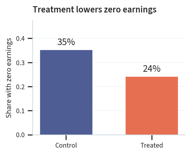
(a) Share with zero earnings.

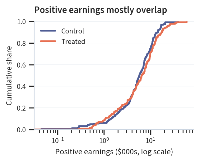
(b) Distribution among positive earners.

Figure 1: Observed earnings in the NSW experimental sample by treatment status. Positive earnings are shown on a logarithmic scale.

Model 1: start with the simplest science

We begin with a model that we already know is wrong.

Earnings cannot be negative, their distribution is strongly right-skewed, and a substantial fraction of workers report exactly zero earnings. A Normal distribution cannot reproduce any of these features. Still, it is a useful place to start. The model is simple enough that we can see every part of the MBPO machinery, from the observed-data likelihood to the imputation of missing potential outcomes. Its failures will also give us a concrete reason to build a better model.

For now, suppose that the potential outcomes follow two Normal distributions:

\begin{pmatrix} Y_i(0) \\ Y_i(1) \end{pmatrix} \mid \theta \sim \mathcal{N}_2 \left[ \begin{pmatrix} \mu_0 \\ \mu_1 \end{pmatrix}, \begin{pmatrix} \sigma_0^2 & 0 \\ 0 & \sigma_1^2 \end{pmatrix} \right],

where \theta=(\mu_0,\mu_1,\sigma_0,\sigma_1). The diagonal covariance matrix implies

\rho = \operatorname{Corr}\left(Y_i(0),Y_i(1)\mid\theta\right)=0.

This is an assumption, not something we learn from the data. As discussed in the theory section on potential-outcome dependence, we never observe Y_i(0) and Y_i(1) for the same worker, so the data identify their marginal distributions but not their association. Setting \rho=0 gives us a convenient baseline. The sensitivity appendix repeats the Model 1 imputation at other fixed values of \rho.

Earnings are measured in thousands of dollars. I use the priors

\begin{aligned} \mu_0 &\sim \mathcal{N}(5,10^2), & \mu_1 &\sim \mathcal{N}(5,10^2),\\ \sigma_0 &\sim \operatorname{HalfNormal}(10), & \sigma_1 &\sim \operatorname{HalfNormal}(10). \end{aligned}

These priors are weakly informative on the scale of the data. The implied prior for the population average treatment effect is

\tau_{\mathrm{pop}}=\mu_1-\mu_0\sim\mathcal{N}(0,2\cdot10^2),

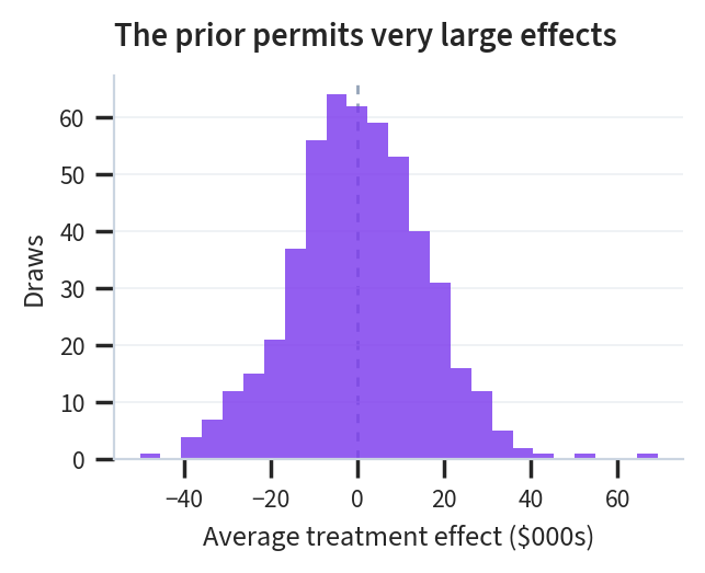
which has a standard deviation of approximately 14.1, or $14,100. The prior permits large positive and negative effects without putting much mass on earnings scales that are completely detached from the application.

Writing the science in NumPyro

The following function handles three distinct operations:

• fit evaluates the observed-data likelihood.
• replicate generates a new dataset under the assignment actually observed in the experiment.
• impute retains the factual outcomes and fills in the missing counterfactuals.

def model1(df, mode="fit"):
    valid_modes = ("fit", "replicate", "impute")
    if mode not in valid_modes:
        raise ValueError(
            f"`mode` must be one of {valid_modes}, got {mode!r}."
        )

    N = df.shape[0]
    w = jnp.asarray(df["treat"].to_numpy(), dtype=bool)
    y = jnp.asarray(df["re78"].to_numpy())

    mu_0 = numpyro.sample("mu_0", dist.Normal(5, 10))
    mu_1 = numpyro.sample("mu_1", dist.Normal(5, 10))
    sig_0 = numpyro.sample("sig_0", dist.HalfNormal(10))
    sig_1 = numpyro.sample("sig_1", dist.HalfNormal(10))

    observed = y if mode == "fit" else None

    with numpyro.plate("unit", N):
        y_0 = numpyro.sample(
            "y_0",
            dist.Normal(mu_0, sig_0).mask(~w),
            obs=observed,
        )
        y_1 = numpyro.sample(
            "y_1",
            dist.Normal(mu_1, sig_1).mask(w),
            obs=observed,
        )

    if mode != "fit":
        q = jnp.array([0.25, 0.50, 0.75])
        numpyro.deterministic("tau_pop", mu_1 - mu_0)
        numpyro.deterministic(
            "tau_qte_pop",
            dist.Normal(mu_1, sig_1).icdf(q)
            - dist.Normal(mu_0, sig_0).icdf(q),
        )

    if mode == "replicate":
        numpyro.deterministic("y_rep", jnp.where(w, y_1, y_0))

    if mode == "impute":
        y_0_imp = numpyro.deterministic(
            "y_0_imp", jnp.where(w, y_0, y)
        )
        y_1_imp = numpyro.deterministic(
            "y_1_imp", jnp.where(w, y, y_1)
        )
        q_y_0_sample = jnp.quantile(y_0_imp, q)
        q_y_1_sample = jnp.quantile(y_1_imp, q)
        numpyro.deterministic(
            "tau_sample", jnp.mean(y_1_imp - y_0_imp)
        )
        numpyro.deterministic(
            "tau_qte_sample", q_y_1_sample - q_y_0_sample
        )

The masks are doing something important. During fitting, both y_0 and y_1 receive the observed earnings vector. The masks determine which elements contribute to the likelihood. The y_0 site contributes

\sum_{i=1}^N (1-W_i)\log\mathcal{N}\left(Y_i^{\mathrm{obs}}\mid\mu_0,\sigma_0^2\right),

while the y_1 site contributes

\sum_{i=1}^N W_i\log\mathcal{N}\left(Y_i^{\mathrm{obs}}\mid\mu_1,\sigma_1^2\right).

Together, they give us the observed-data likelihood

p(\mathbf Y^{\mathrm{obs}}\mid\theta,\mathbf W) = \prod_{i:W_i=0}p(Y_i^{\mathrm{obs}}\mid\mu_0,\sigma_0) \prod_{i:W_i=1}p(Y_i^{\mathrm{obs}}\mid\mu_1,\sigma_1).

The missing potential outcomes have already been integrated out. They do not enter the NUTS state. We could write the same likelihood with a single observed distribution whose location and scale are selected with jnp.where. The two forms are algebraically equivalent. I prefer the masked version here because it keeps the two potential-outcome distributions visible in the code. That is the science we are trying to model.

Prior predictive checks

Before fitting the model, we simulate earnings distributions from the prior. In replicate mode, the model generates both potential outcomes and then applies the observed assignment:

Y_i^{\mathrm{rep}}=W_iY_i^{\mathrm{rep}}(1)+(1-W_i)Y_i^{\mathrm{rep}}(0).

No observed earnings enter this calculation. At this stage I am asking two fairly narrow questions: does the prior put earnings on a remotely sensible scale, and what range of treatment effects does it imply before seeing the outcomes?

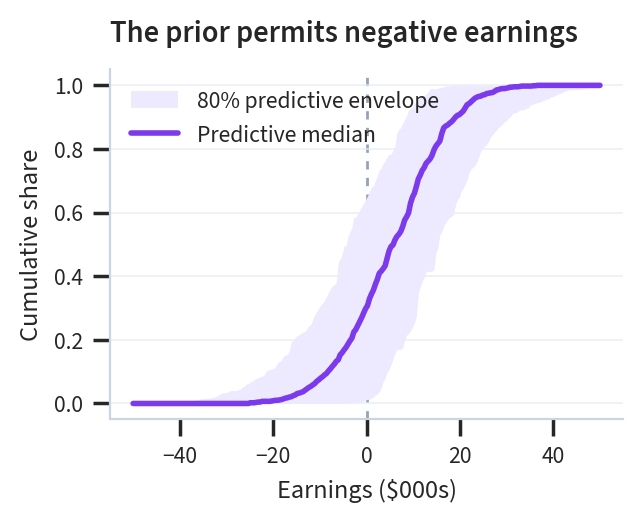
As Figure 2 shows, the prior predictive distribution is broad but remains on a recognizable earnings scale. It also exposes a problem that no reasonable choice of parameters can repair: the Normal model assigns positive probability to negative earnings. This is a failure of the outcome family, not simply a failure of the prior. Tightening the priors could reduce the number of negative draws, but it cannot make the support of the model agree with the support of the outcome.

key, prior_key = jr.split(jr.PRNGKey(235))
prior_predictive_m1 = infer.Predictive(
    model1,
    num_samples=500,
    return_sites=["y_rep", "tau_pop", "tau_qte_pop"],
)
prior_samples_m1 = prior_predictive_m1(
    prior_key,
    df=df,
    mode="replicate",
)
y_prior_samples_m1 = np.asarray(prior_samples_m1["y_rep"])

# hide-code-pdf-source: paired-with-cell-class

fig, ax = plt.subplots(figsize=(3.1, 2.5))
plot_predictive_ecdf(
    y_prior_samples_m1[:100],
    stage="prior",
    grid=np.linspace(-50, 50, 240),
    ax=ax,
)
add_reference_line(ax)
ax.set_xlabel("Earnings ($000s)")
ax.set_ylabel("Cumulative share")
ax.set_title("The prior permits negative earnings")
ax.legend(title=None)
plt.show()

tau_prior_samples_m1 = np.asarray(prior_samples_m1["tau_pop"])
fig, ax = plt.subplots(figsize=(3.1, 2.5))
plot_histogram(tau_prior_samples_m1, color=COLORS["prior"], bins=25, ax=ax)
add_reference_line(ax)
ax.set_xlabel("Average treatment effect ($000s)")
ax.set_ylabel("Draws")
ax.set_title("The prior permits very large effects")
plt.show()

(a) Outcome distribution.

(b) Average treatment effect.

Figure 2: Prior predictive implications under the Normal model. The first panel shows the median ECDF and central 80% envelope across 100 replicated datasets; the second uses 500 prior ATE draws.

Fitting the observed-data model

We fit the model with four NUTS chains. Because the missing potential outcomes have been marginalized, the sampler needs to explore only the four-dimensional parameter vector \theta.

key, fit_key = jr.split(key)
nb_samples = 1_000
kernel_m1 = infer.NUTS(model1)
sampler_m1 = infer.MCMC(
    kernel_m1,
    num_samples=nb_samples,
    num_warmup=1_000,
    num_chains=4,
    chain_method="sequential",
    progress_bar=False,
)

sampler_m1.run(fit_key, df=df, mode="fit")
sampler_m1.print_summary()

posterior_samples_m1 = sampler_m1.get_samples()

                mean       std    median      5.0%     95.0%     n_eff     r_hat
      mu_0      4.56      0.34      4.56      4.00      5.11   3878.26      1.00
      mu_1      6.34      0.59      6.34      5.36      7.32   4377.51      1.00
     sig_0      5.51      0.25      5.51      5.11      5.90   4619.56      1.00
     sig_1      7.90      0.41      7.89      7.25      8.61   4375.90      1.00

Number of divergences: 0

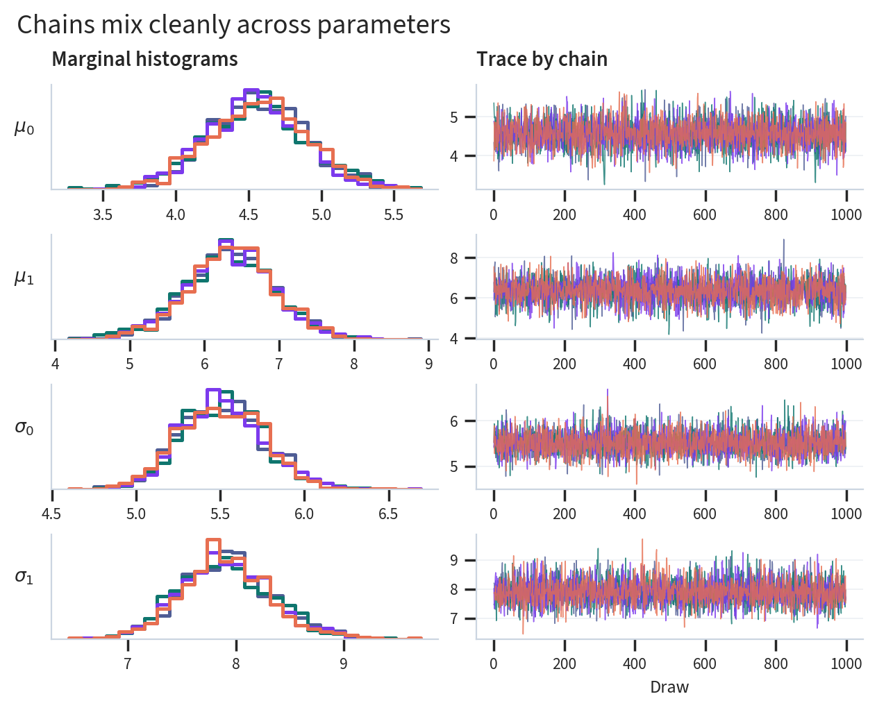
The sampler behaves well. There are no divergent transitions, the rank-normalized \widehat R values are essentially one, and the effective sample sizes are large relative to the number of retained draws. The posterior means are approximately

\begin{aligned} \mathbb{E}[\mu_0\mid\text{data}] &\approx 4.56, & \mathbb{E}[\mu_1\mid\text{data}] &\approx 6.34,\\ \mathbb{E}[\sigma_0\mid\text{data}] &\approx 5.51, & \mathbb{E}[\sigma_1\mid\text{data}] &\approx 7.90. \end{aligned}

The model estimates higher average earnings under treatment, together with substantially greater dispersion. The corresponding calculation in Chapter 8 gives the same broad result: an average effect around $1,800 and posterior uncertainty around $500 for the finite-sample estimand. I use that comparison as an implementation check rather than as a separate result.

m1_idata = az.from_numpyro(sampler_m1)
az.summary(
    m1_idata,
    var_names=["mu_0", "mu_1", "sig_0", "sig_1"],
)

	mean	sd	eti89_lb	eti89_ub	ess_bulk	ess_tail	r_hat	mcse_mean	mcse_sd
mu_0	4.56	0.341	4	5.1	3900	3120	1.00	0.0055	0.004
mu_1	6.34	0.59	5.4	7.3	4391	3218	1.00	0.0089	0.0065
sig_0	5.511	0.247	5.1	5.9	4688	3053	1.00	0.0036	0.0026
sig_1	7.9	0.414	7.3	8.6	4431	2928	1.00	0.0063	0.0045

trace_samples_m1 = sampler_m1.get_samples(group_by_chain=True)
trace_parameters_m1 = [
    ("mu_0", r"$\mu_0$"),
    ("mu_1", r"$\mu_1$"),
    ("sig_0", r"$\sigma_0$"),
    ("sig_1", r"$\sigma_1$"),
]
chain_colors = [
    COLORS["control"],
    COLORS["posterior"],
    COLORS["prior"],
    COLORS["treated"],
]

fig, axes = plt.subplots(4, 2, figsize=(6.2, 5.0))
for row, (parameter, label) in enumerate(trace_parameters_m1):
    values = np.asarray(trace_samples_m1[parameter])
    parameter_bins = np.histogram_bin_edges(values.ravel(), bins=28)
    for chain, color in enumerate(chain_colors):
        plot_step_histogram(
            values[chain],
            color=color,
            bins=parameter_bins,
            ax=axes[row, 0],
        )
        axes[row, 1].plot(
            values[chain],
            color=color,
            linewidth=0.55,
            alpha=0.8,
        )
    axes[row, 0].set_ylabel(label, rotation=0, labelpad=14)
    axes[row, 0].set_yticks([])
    axes[row, 1].set_ylabel("")
    if row < len(trace_parameters_m1) - 1:
        axes[row, 0].set_xlabel("")
        axes[row, 1].set_xlabel("")

axes[0, 0].set_title("Marginal histograms")
axes[0, 1].set_title("Trace by chain")
axes[-1, 1].set_xlabel("Draw")
fig.suptitle("Chains mix cleanly across parameters", x=0.01, ha="left")
plt.show()

Figure 3: Each color identifies one NUTS chain. Step histograms show unsmoothed marginal distributions; trace panels show 1,000 post-warmup draws per chain.

Posterior predictive checks

Good computational diagnostics tell us that NUTS successfully sampled from the posterior we specified. They do not tell us whether that posterior arises from a useful model of earnings. For that, we generate replicated datasets using mode="replicate".

Conditional on a posterior draw,

Y_i^{\mathrm{rep}}\sim\mathcal{N}\left(\mu_{W_i},\sigma_{W_i}^2\right).

The comparison should be made separately by treatment status, since the model assigns each arm a different distribution. A density overlay is useful, but it can hide the most important failures. I also compare the fraction of workers with exactly zero earnings,

T_0(\mathbf Y)=\frac{1}{N}\sum_{i=1}^N\mathbf{1}(Y_i=0),

the fraction with negative earnings,

T_-(\mathbf Y)=\frac{1}{N}\sum_{i=1}^N\mathbf{1}(Y_i<0),

and statistics that describe the right tail.

key, ppc_key = jr.split(key)
posterior_predictive_m1 = infer.Predictive(
    model1,
    posterior_samples=posterior_samples_m1,
    return_sites=["y_rep"],
)
ppc_m1 = posterior_predictive_m1(
    ppc_key,
    df=df,
    mode="replicate",
)

def sample_skewness(x, axis=-1):
    centered = x - np.mean(x, axis=axis, keepdims=True)
    scale = np.std(x, axis=axis)
    return np.mean(centered**3, axis=axis) / scale**3

def ppc_statistic_table(y_obs, y_rep, arm):
    statistics = {
        "Share equal to zero": (np.mean(y_obs == 0), np.mean(y_rep == 0, axis=1)),
        "Share below zero": (np.mean(y_obs < 0), np.mean(y_rep < 0, axis=1)),
        "90th percentile": (np.quantile(y_obs, 0.90), np.quantile(y_rep, 0.90, axis=1)),
        "Skewness": (sample_skewness(y_obs), sample_skewness(y_rep)),
    }
    return pl.DataFrame(
        [
            {
                "arm": arm,
                "statistic": name,
                "observed": observed,
                "predictive_median": np.median(draws),
                "predictive_05": np.quantile(draws, 0.05),
                "predictive_95": np.quantile(draws, 0.95),
            }
            for name, (observed, draws) in statistics.items()
        ]
    )

w_m1 = df["treat"].to_numpy().astype(bool)
y_m1 = df["re78"].to_numpy()
y_rep_m1 = np.asarray(ppc_m1["y_rep"])
ppc_summary_m1 = pl.concat(
    [
        ppc_statistic_table(y_m1[~w_m1], y_rep_m1[:, ~w_m1], "Control"),
        ppc_statistic_table(y_m1[w_m1], y_rep_m1[:, w_m1], "Treated"),
    ]
)
ppc_summary_m1.style.fmt_number(
    columns=["observed", "predictive_median", "predictive_05", "predictive_95"],
    decimals=2,
)

arm	statistic	observed	predictive_median	predictive_05	predictive_95
Control	Share equal to zero	0.35	0.00	0.00	0.00
Control	Share below zero	0.00	0.20	0.15	0.26
Control	90th percentile	11.36	11.55	10.35	12.77
Control	Skewness	1.82	0.00	−0.26	0.24
Treated	Share equal to zero	0.24	0.00	0.00	0.00
Treated	Share below zero	0.00	0.21	0.15	0.28
Treated	90th percentile	14.55	16.34	14.31	18.50
Treated	Skewness	2.72	−0.00	−0.29	0.29

# hide-code-pdf-source: paired-with-cell-class
fig_control_m1, ax_control_m1 = plt.subplots(figsize=(3.1, 2.5))
fig_treated_m1, ax_treated_m1 = plt.subplots(figsize=(3.1, 2.5))
plot_posterior_predictive_by_arm(
    y_m1,
    y_rep_m1[:100],
    w_m1,
    axes=(ax_control_m1, ax_treated_m1),
    title="Zeros break the Normal fit",
)
plt.show()

(a) Control.

(b) Treated.

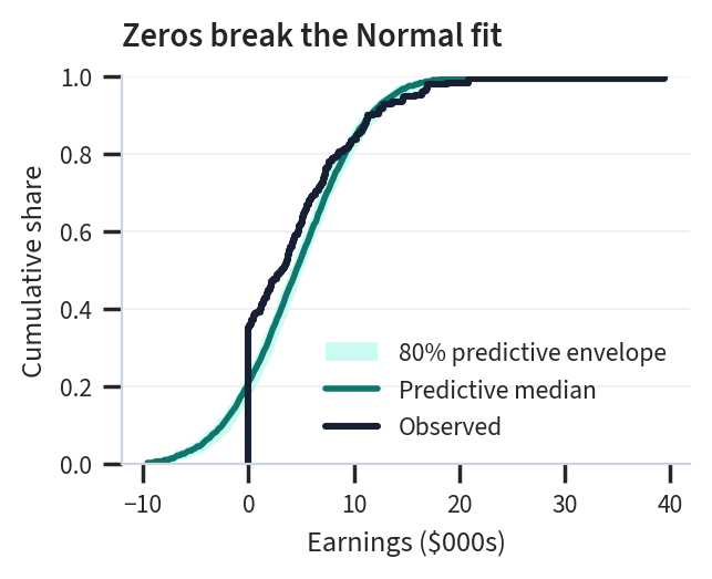
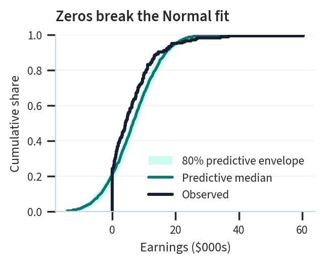
Figure 4: Black lines show observed ECDFs; teal lines and mint bands show posterior predictive medians and central 80% envelopes across 100 replicated datasets.

The diagnosis is unambiguous. The observed data contain a large point mass at zero, while a continuous Normal distribution produces zero with probability zero. The replicated datasets contain negative earnings and are symmetric, while positive earnings are strongly right-skewed. The model can reproduce the arm-specific means and variances, but not the shape of either distribution.

The distinction between a prior and a posterior failure is useful here. Before fitting, we saw that the model could generate negative earnings. After fitting, we see that the problem has not disappeared and that the model also cannot reproduce the bunching at zero or the right tail.

The next step is not to tighten the priors. It is also not obvious that adding covariates would solve the problem. Neither change would repair the support of the outcome distribution. We need to revise the science model for earnings.

Imputing the missing potential outcomes

Posterior predictive replication asks whether the fitted model can reproduce data like those we observed. Causal imputation asks a different question: what does the fitted model imply about the potential outcomes we did not observe? We keep these two operations separate in the code.

key, imputation_key = jr.split(key)
posterior_imputation_m1 = infer.Predictive(
    model1,
    posterior_samples=posterior_samples_m1,
    return_sites=[
        "y_0_imp",
        "y_1_imp",
        "tau_pop",
        "tau_sample",
        "tau_qte_pop",
        "tau_qte_sample",
    ],
)
imputations_m1 = posterior_imputation_m1(
    imputation_key,
    df=df,
    mode="impute",
)

For each posterior draw \theta^{(s)}, the baseline model imputes

Y_i^{\mathrm{mis}}(0)\sim\mathcal{N}\left(\mu_0^{(s)},(\sigma_0^{(s)})^2\right)

for treated workers, and

Y_i^{\mathrm{mis}}(1)\sim\mathcal{N}\left(\mu_1^{(s)},(\sigma_1^{(s)})^2\right)

for control workers. We then complete each potential-outcome schedule:

Y_i^{\mathrm{imp}}(0)= \begin{cases} Y_i^{\mathrm{obs}}, & W_i=0,\\ Y_i^{\mathrm{mis}}(0), & W_i=1, \end{cases} \qquad Y_i^{\mathrm{imp}}(1)= \begin{cases} Y_i^{\mathrm{mis}}(1), & W_i=0,\\ Y_i^{\mathrm{obs}}, & W_i=1. \end{cases}

Each posterior draw gives us one completed schedule of potential outcomes. We can calculate any finite-sample causal estimand from that schedule.

Population and finite-sample estimands

The population average treatment effect is

\tau_{\mathrm{pop}}=\mathbb{E}[Y(1)-Y(0)\mid\theta]=\mu_1-\mu_0.

Its posterior mean is approximately 1.78, or $1,780, with a posterior standard deviation of 0.69. The central 90 percent credible interval is approximately [0.66,2.90].

For the workers in the experiment, the finite-sample average treatment effect is

\tau_{\mathrm{sample}}=\frac{1}{N}\sum_{i=1}^N\left[Y_i^{\mathrm{imp}}(1)-Y_i^{\mathrm{imp}}(0)\right].

Its posterior mean is approximately 1.80, with a posterior standard deviation of 0.50. The population and sample averages are similar in this application, but they are different estimands and need not agree in general.

effects_m1 = pl.DataFrame(
    {
        "tau_pop": np.asarray(imputations_m1["tau_pop"]),
        "tau_sample": np.asarray(imputations_m1["tau_sample"]),
        "tau_q25_sample": np.asarray(imputations_m1["tau_qte_sample"])[:, 0],
        "tau_q50_sample": np.asarray(imputations_m1["tau_qte_sample"])[:, 1],
        "tau_q75_sample": np.asarray(imputations_m1["tau_qte_sample"])[:, 2],
        "tau_q25_pop": np.asarray(imputations_m1["tau_qte_pop"])[:, 0],
        "tau_q50_pop": np.asarray(imputations_m1["tau_qte_pop"])[:, 1],
        "tau_q75_pop": np.asarray(imputations_m1["tau_qte_pop"])[:, 2],
    }
)
effects_description_specs_m1 = [
    ("ATE summaries", ["tau_pop", "tau_sample"]),
    (
        "Finite-sample QTE summaries",
        ["tau_q25_sample", "tau_q50_sample", "tau_q75_sample"],
    ),
    (
        "Population QTE summaries",
        ["tau_q25_pop", "tau_q50_pop", "tau_q75_pop"],
    ),
]
for title, columns in effects_description_specs_m1:
    display({"text/markdown": f"**{title}**"}, raw=True)
    display(
        effects_m1.select(columns).describe().style.fmt_number(
            columns=columns, decimals=2
        )
    )

ATE summaries

statistic	tau_pop	tau_sample
count	4,000.00	4,000.00
null_count	0.00	0.00
mean	1.78	1.80
std	0.69	0.50
min	−1.02	−0.01
25%	1.33	1.47
50%	1.79	1.80
75%	2.25	2.13
max	4.04	3.52

Finite-sample QTE summaries

statistic	tau_q25_sample	tau_q50_sample	tau_q75_sample
count	4,000.00	4,000.00	4,000.00
null_count	0.00	0.00	0.00
mean	0.62	1.64	3.09
std	0.35	0.56	0.64
min	−0.13	−0.12	0.84
25%	0.47	1.26	2.66
50%	0.65	1.63	3.12
75%	0.82	2.02	3.52
max	2.00	3.65	5.34

Population QTE summaries

statistic	tau_q25_pop	tau_q50_pop	tau_q75_pop
count	4,000.00	4,000.00	4,000.00
null_count	0.00	0.00	0.00
mean	0.17	1.78	3.40
std	0.75	0.69	0.77
min	−2.87	−1.02	0.55
25%	−0.32	1.33	2.88
50%	0.19	1.79	3.40
75%	0.68	2.25	3.92
max	2.61	4.04	6.20

completed_y0_m1 = np.asarray(imputations_m1["y_0_imp"])[:10].ravel()
completed_y1_m1 = np.asarray(imputations_m1["y_1_imp"])[:10].ravel()
completed_bins_m1 = np.histogram_bin_edges(
    np.concatenate([completed_y0_m1, completed_y1_m1]),
    bins=32,
)

fig, ax = plt.subplots(figsize=(5.8, 3.1))
plot_step_histogram(
    completed_y0_m1,
    label=r"Control potential outcome $Y(0)$",
    color=COLORS["control"],
    bins=completed_bins_m1,
    ax=ax,
)
plot_step_histogram(
    completed_y1_m1,
    label=r"Treatment potential outcome $Y(1)$",
    color=COLORS["treated"],
    bins=completed_bins_m1,
    ax=ax,
)
ax.set_xlabel("Completed earnings ($000s)")
ax.set_ylabel("Density")
ax.set_title("Treatment shifts completed earnings right")
ax.legend(title=None)
plt.show()

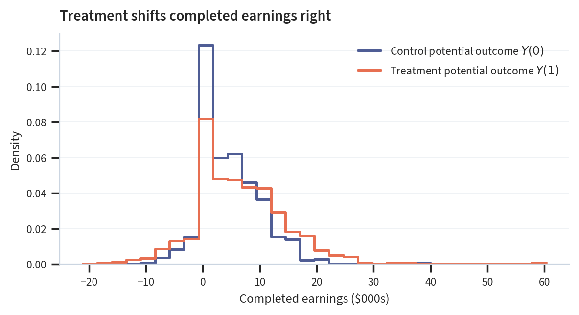
Figure 5: Unsmoothed density histograms pool the first 10 completed potential-outcome schedules from Model 1. Negative earnings remain possible under the Normal outcome family.

We can also calculate population quantile treatment effects. For quantile q,

\tau_q^{\mathrm{pop}}=Q_q\{Y(1)\}-Q_q\{Y(0)\}.

Because the two marginal distributions are Normal,

\tau_q^{\mathrm{pop}}=(\mu_1-\mu_0)+(\sigma_1-\sigma_0)\Phi^{-1}(q).

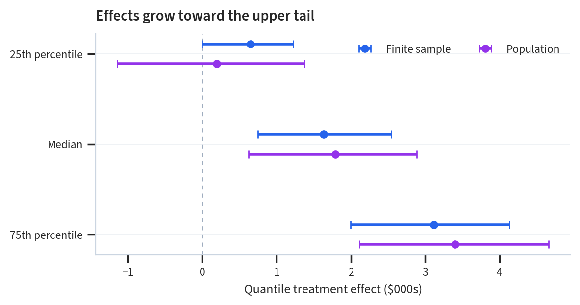
The posterior means at the first quartile, median, and third quartile are approximately 0.17, 1.78, and 3.40. For the completed experimental sample, the corresponding posterior means are approximately 0.62, 1.64, and 3.09.

The population and finite-sample QTEs differ because the latter retain the observed outcomes, including their large point mass at zero, and impute only the missing outcomes. The increasing population QTE is driven by the larger estimated variance under treatment. It should not yet receive a strong substantive interpretation. The Normal model is attempting to explain a point-mass, right-skewed outcome through changes in only its mean and variance.

These completed schedules use the baseline assumption \rho=0. The observed data cannot select that value. The sensitivity appendix shows how the finite-sample conclusions change when the same Model 1 marginals are paired using other fixed correlations.

q_labels = ["25th percentile", "Median", "75th percentile"]
qte_sample_m1 = np.asarray(imputations_m1["tau_qte_sample"])
qte_pop_m1 = np.asarray(imputations_m1["tau_qte_pop"])

fig, ax = plt.subplots(figsize=(5.8, 3.0))
y_positions = np.arange(len(q_labels))
for draws, label, color, offset in [
    (qte_sample_m1, "Finite sample", COLORS["sample"], -0.11),
    (qte_pop_m1, "Population", COLORS["population"], 0.11),
]:
    lower, median, upper = np.quantile(draws, [0.05, 0.50, 0.95], axis=0)
    ax.errorbar(
        median,
        y_positions + offset,
        xerr=np.vstack([median - lower, upper - median]),
        fmt="o",
        color=color,
        elinewidth=2,
        capsize=3,
        markersize=5,
        label=label,
    )
add_reference_line(ax)
ax.set_yticks(y_positions, q_labels)
ax.invert_yaxis()
ax.set_xlabel("Quantile treatment effect ($000s)")
ax.set_ylabel("")
ax.set_title("Effects grow toward the upper tail")
ax.legend(title=None, ncol=2, loc="upper right")
plt.show()

Figure 6: Points are posterior medians and whiskers are central 90% intervals. Finite-sample QTEs use completed potential-outcome schedules; population QTEs use the fitted Normal marginals.

What we learned from Model 1

Model 1 has done useful work. It gave us a transparent implementation of MBPO, showed how masking produces the marginalized observed-data likelihood, and separated posterior predictive replication from causal imputation. It also produced a baseline estimate of the average treatment effect.

More importantly, it failed its predictive checks in ways that are directly connected to the economics of earnings. The data contain a positive-earnings margin, represented by the point mass at zero, and a highly skewed distribution among positive earners. A Normal model has neither feature.

The natural repair is a hurdle model with one process for whether earnings are positive and another for their level conditional on being positive. Before making that change, I first add covariates while holding the Normal likelihood fixed. This controlled comparison shows what covariates can and cannot repair.

Model 2: hold the Normal likelihood fixed and add covariates

The first revision changes only the conditional means. For w\in\{0,1\},

Y_i(w)\mid\mathbf{X}_i,\theta \sim\mathcal{N}\!\left(\mu_w+\mathbf{X}_i^\top\beta_w,\sigma_w^2\right).

Separate coefficient vectors allow the conditional mean effect

\tau_i^X(\theta) =\mathbb{E}\{Y_i(1)-Y_i(0)\mid\mathbf{X}_i,\theta\} =(\mu_1-\mu_0)+\mathbf{X}_i^\top(\beta_1-\beta_0)

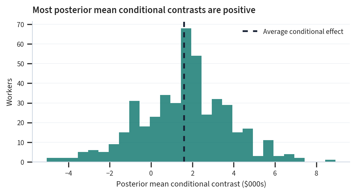
to vary with the observed covariate profile. This is a conditional mean contrast, not a realized individual treatment effect. The realized contrast Y_i(1)-Y_i(0) still depends on two potential outcomes that are never jointly observed.

I standardize age, educ, re74, and re75, and leave the five binary indicators black, married, nodegr, u74, and u75 as 0/1. These are the nine regressors in the Chapter 8 two-part specification; the intercept is a separate parameter. The design matrix therefore has nine columns, not ten, and does not include hisp.

The priors retain the scale of Model 1:

\begin{aligned} \mu_w&\sim\mathcal{N}(5,10^2), & \beta_{wk}&\sim\mathcal{N}(0,3^2), & \sigma_w&\sim\operatorname{HalfNormal}(10). \end{aligned}

Averaging the conditional mean contrasts over the observed covariate profiles gives the sample-standardized estimand \tau^X from Equation 10. Imputing the missing potential outcomes gives the realized finite-sample estimand \tau^S. Keeping those calculations separate prevents a regression contrast from being mislabeled as an individual causal effect.

x_cont = ["age", "educ", "re74", "re75"]
x_bin = ["black", "married", "nodegr", "u74", "u75"]
x_names = x_cont + x_bin

X_cont = df.select(x_cont).to_numpy().astype(float)
X_cont = (X_cont - X_cont.mean(0)) / X_cont.std(0)
X_bin = df.select(x_bin).to_numpy().astype(float)
X = np.hstack([X_cont, X_bin])

assert X.shape == (df.height, 9)
assert x_names == [
    "age", "educ", "re74", "re75", "black",
    "married", "nodegr", "u74", "u75",
]

def model2(df, X, mode="fit"):
    valid_modes = ("fit", "replicate", "impute")
    if mode not in valid_modes:
        raise ValueError(f"`mode` must be one of {valid_modes}, got {mode!r}.")

    N, K = X.shape
    w = jnp.asarray(df["treat"].to_numpy(), dtype=bool)
    y = jnp.asarray(df["re78"].to_numpy())
    Xj = jnp.asarray(X)

    mu_0 = numpyro.sample("mu_0", dist.Normal(5, 10))
    mu_1 = numpyro.sample("mu_1", dist.Normal(5, 10))
    beta_0 = numpyro.sample("beta_0", dist.Normal(0, 3).expand([K]))
    beta_1 = numpyro.sample("beta_1", dist.Normal(0, 3).expand([K]))
    sig_0 = numpyro.sample("sig_0", dist.HalfNormal(10))
    sig_1 = numpyro.sample("sig_1", dist.HalfNormal(10))

    loc_0 = mu_0 + Xj @ beta_0
    loc_1 = mu_1 + Xj @ beta_1
    observed = y if mode == "fit" else None

    with numpyro.plate("unit", N):
        y_0 = numpyro.sample(
            "y_0", dist.Normal(loc_0, sig_0).mask(~w), obs=observed
        )
        y_1 = numpyro.sample(
            "y_1", dist.Normal(loc_1, sig_1).mask(w), obs=observed
        )

    if mode != "fit":
        tau_cond = numpyro.deterministic("tau_cond", loc_1 - loc_0)
        numpyro.deterministic("tau_x", jnp.mean(tau_cond))

    if mode == "replicate":
        numpyro.deterministic("y_rep", jnp.where(w, y_1, y_0))

    if mode == "impute":
        q = jnp.array([0.25, 0.50, 0.75])
        y_0_imp = numpyro.deterministic("y_0_imp", jnp.where(w, y_0, y))
        y_1_imp = numpyro.deterministic("y_1_imp", jnp.where(w, y, y_1))
        numpyro.deterministic("tau_sample", jnp.mean(y_1_imp - y_0_imp))
        numpyro.deterministic(
            "tau_qte_sample",
            jnp.quantile(y_1_imp, q) - jnp.quantile(y_0_imp, q),
        )

Prior predictive checks

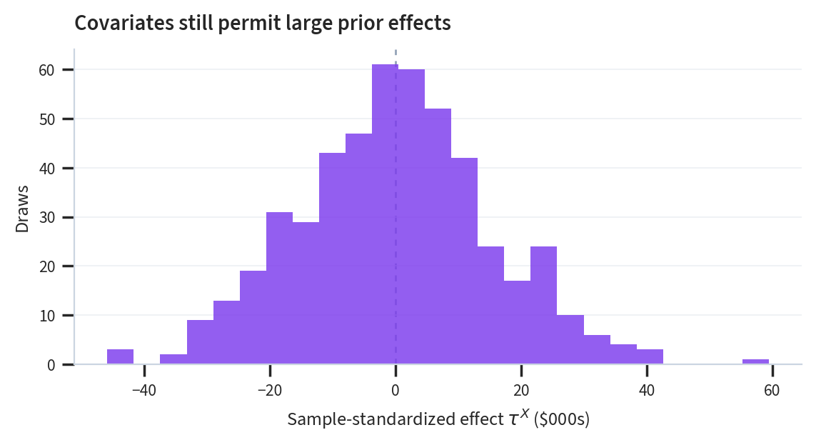
I first run the model in replicate mode without conditioning on the outcomes. The same targeted statistics used for Model 1 reveal what the priors and the Normal likelihood imply jointly: the share at zero, the share below zero, the 90th percentile, and skewness, all calculated separately by treatment status. I also inspect the prior distribution of \tau^X.

Adding covariates does not change the support of the model. Prior predictive datasets can still contain negative earnings, and an exactly zero outcome still has probability zero. The point of this check is therefore not to confirm that the Normal model has become realistic. It is to verify that the regression priors imply plausible conditional mean variation before fitting.

key, prior_key_m2 = jr.split(key)
prior_predictive_m2 = infer.Predictive(
    model2,
    num_samples=500,
    return_sites=["y_rep", "tau_x"],
)
prior_samples_m2 = prior_predictive_m2(
    prior_key_m2, df=df, X=X, mode="replicate"
)
y_prior_m2 = np.asarray(prior_samples_m2["y_rep"])

prior_checks_m2 = ppc_statistic_table(
    y_m1[~w_m1], y_prior_m2[:, ~w_m1], "Control"
).vstack(
    ppc_statistic_table(y_m1[w_m1], y_prior_m2[:, w_m1], "Treated")
)
display(
    prior_checks_m2.style.fmt_number(
        columns=[
            "observed", "predictive_median", "predictive_05", "predictive_95"
        ],
        decimals=2,
    )
)

arm	statistic	observed	predictive_median	predictive_05	predictive_95
Control	Share equal to zero	0.35	0.00	0.00	0.00
Control	Share below zero	0.00	0.35	0.00	0.96
Control	90th percentile	11.36	16.85	−2.87	41.12
Control	Skewness	1.82	−0.00	−1.46	1.33
Treated	Share equal to zero	0.24	0.00	0.00	0.00
Treated	Share below zero	0.00	0.33	0.01	0.94
Treated	90th percentile	14.55	17.47	−1.49	38.53
Treated	Skewness	2.72	0.01	−1.16	1.15

fig, ax = plt.subplots(figsize=(5.6, 3.0))
plot_histogram(
    np.asarray(prior_samples_m2["tau_x"]),
    color=COLORS["prior"],
    bins=25,
    ax=ax,
)
add_reference_line(ax)
ax.set_xlabel(r"Sample-standardized effect $\tau^X$ (\$000s)")
ax.set_ylabel("Draws")
ax.set_title("Covariates still permit large prior effects")
plt.show()

Figure 7: The sample-standardized prior effect integrates Model 2’s covariate-specific contrasts over the observed covariate distribution. The histogram contains 500 prior draws.

Fitting the observed-data model

Fitting again uses the marginalized observed-data likelihood. The only additional unknowns are the arm-specific regression coefficients. I check divergences, \widehat R, and effective sample sizes before interpreting either the regression contrasts or the imputed potential outcomes.

key, fit_key_m2 = jr.split(key)
sampler_m2 = infer.MCMC(
    infer.NUTS(model2),
    num_samples=1_000,
    num_warmup=1_000,
    num_chains=4,
    chain_method="sequential",
    progress_bar=False,
)
sampler_m2.run(fit_key_m2, df=df, X=X, mode="fit")
# sampler_m2.print_summary(exclude_deterministic=True)
posterior_samples_m2 = sampler_m2.get_samples()

m2_idata = az.from_numpyro(
    sampler_m2,
    coords={"covariate": x_names},
    dims={"beta_0": ["covariate"], "beta_1": ["covariate"]},
)
az.summary(
    m2_idata,
    var_names=["mu_0", "mu_1", "beta_0", "beta_1", "sig_0", "sig_1"],
)

	mean	sd	eti89_lb	eti89_ub	ess_bulk	ess_tail	r_hat	mcse_mean	mcse_sd
mu_0	8.02	1.38	5.8	10	3764	3046	1.00	0.023	0.016
mu_1	5.58	1.94	2.5	8.7	4031	2886	1.00	0.03	0.021
beta_0[age]	0.266	0.343	-0.28	0.81	6832	3176	1.00	0.0041	0.0028
beta_0[educ]	0.19	0.468	-0.57	0.93	4681	3543	1.00	0.0068	0.0049
beta_0[re74]	0.04	0.47	-0.73	0.78	4367	3316	1.00	0.0071	0.005
beta_0[re75]	0	0.51	-0.78	0.81	4998	3115	1.00	0.0072	0.0052
beta_0[black]	-2.35	0.87	-3.7	-0.95	5712	3149	1.00	0.012	0.0082
beta_0[married]	-0.73	0.93	-2.3	0.73	5546	2984	1.00	0.013	0.0087
beta_0[nodegr]	-0.12	1.07	-1.9	1.6	3989	3103	1.00	0.017	0.012
beta_0[u74]	-2.15	1.19	-4.1	-0.29	4233	2951	1.00	0.018	0.013
beta_0[u75]	0.48	1.01	-1.1	2.1	4756	3119	1.00	0.015	0.0099
beta_1[age]	0.45	0.58	-0.48	1.4	6579	3162	1.00	0.0071	0.0052
beta_1[educ]	1.03	0.63	0.022	2	4857	3352	1.00	0.009	0.0065
beta_1[re74]	0.99	0.88	-0.43	2.4	4621	3116	1.00	0.013	0.0092
beta_1[re75]	0.24	0.79	-0.98	1.5	5184	3155	1.00	0.011	0.0075
beta_1[black]	-0.91	1.38	-3.1	1.3	5948	3232	1.00	0.018	0.013
beta_1[married]	0.81	1.38	-1.3	3.1	6820	3437	1.00	0.017	0.012
beta_1[nodegr]	-0.52	1.48	-2.9	1.8	4348	3506	1.00	0.022	0.016
beta_1[u74]	4.1	1.71	1.4	6.8	4095	2836	1.00	0.027	0.019
beta_1[u75]	-2.12	1.54	-4.5	0.4	4734	2847	1.00	0.022	0.016
sig_0	5.415	0.246	5	5.8	6839	2934	1.00	0.003	0.0021
sig_1	7.68	0.414	7.1	8.4	6458	3262	1.00	0.0052	0.0041

Posterior predictive checks and causal imputation

The computation is well behaved: there are no divergent transitions, every reported \widehat R rounds to 1.00, and the effective sample sizes are comfortably large.

I now use the fitted model twice for two different purposes. In replicate mode, it generates new observed datasets for checking the Normal regression. In impute mode, it combines the factual outcomes with simulated counterfactuals to complete the potential-outcome schedule. The first operation diagnoses the model; the second propagates its assumptions into the causal estimands.

key, ppc_key_m2, imputation_key_m2 = jr.split(key, 3)

posterior_predictive_m2 = infer.Predictive(
    model2,
    posterior_samples=posterior_samples_m2,
    return_sites=["y_rep", "tau_cond", "tau_x"],
)
ppc_m2 = posterior_predictive_m2(
    ppc_key_m2, df=df, X=X, mode="replicate"
)
y_rep_m2 = np.asarray(ppc_m2["y_rep"])
ppc_summary_m2 = pl.concat(
    [
        ppc_statistic_table(y_m1[~w_m1], y_rep_m2[:, ~w_m1], "Control"),
        ppc_statistic_table(y_m1[w_m1], y_rep_m2[:, w_m1], "Treated"),
    ]
)
display(
    ppc_summary_m2.style.fmt_number(
        columns=[
            "observed", "predictive_median", "predictive_05", "predictive_95"
        ],
        decimals=2,
    )
)

posterior_imputation_m2 = infer.Predictive(
    model2,
    posterior_samples=posterior_samples_m2,
    return_sites=[
        "y_0_imp", "y_1_imp", "tau_cond", "tau_x",
        "tau_sample", "tau_qte_sample",
    ],
)
imputations_m2 = posterior_imputation_m2(
    imputation_key_m2, df=df, X=X, mode="impute"
)

effects_m2 = pl.DataFrame(
    {
        "tau_x": np.asarray(imputations_m2["tau_x"]),
        "tau_sample": np.asarray(imputations_m2["tau_sample"]),
        "tau_q25_sample": np.asarray(imputations_m2["tau_qte_sample"])[:, 0],
        "tau_q50_sample": np.asarray(imputations_m2["tau_qte_sample"])[:, 1],
        "tau_q75_sample": np.asarray(imputations_m2["tau_qte_sample"])[:, 2],
    }
)
effect_labels_m2 = {
    "tau_x": r"Sample-standardized mean effect $\tau^X$",
    "tau_sample": r"Finite-sample ATE $\tau^S$",
    "tau_q25_sample": "Finite-sample QTE, 25th percentile",
    "tau_q50_sample": "Finite-sample QTE, median",
    "tau_q75_sample": "Finite-sample QTE, 75th percentile",
}
effects_summary_m2 = pl.DataFrame(
    [
    {
            "estimand": label,
            "mean": np.mean(draws),
            "sd": np.std(draws),
            "p05": np.quantile(draws, 0.05),
            "p50": np.quantile(draws, 0.50),
            "p95": np.quantile(draws, 0.95),
        }
        for name, label in effect_labels_m2.items()
        for draws in [effects_m2[name].to_numpy()]
    ]
)
display(
    effects_summary_m2.style.fmt_number(
        columns=["mean", "sd", "p05", "p50", "p95"], decimals=2
    )
)

arm	statistic	observed	predictive_median	predictive_05	predictive_95
Control	Share equal to zero	0.35	0.00	0.00	0.00
Control	Share below zero	0.00	0.21	0.16	0.27
Control	90th percentile	11.36	11.71	10.55	12.97
Control	Skewness	1.82	0.02	−0.23	0.26
Treated	Share equal to zero	0.24	0.00	0.00	0.00
Treated	Share below zero	0.00	0.22	0.16	0.28
Treated	90th percentile	14.55	16.57	14.70	18.71
Treated	Skewness	2.72	0.01	−0.29	0.30

estimand	mean	sd	p05	p50	p95
Sample-standardized mean effect $\tau^X$	1.59	0.66	0.50	1.60	2.69
Finite-sample ATE $\tau^S$	1.59	0.49	0.78	1.59	2.39
Finite-sample QTE, 25th percentile	0.47	0.34	0.00	0.55	1.05
Finite-sample QTE, median	1.43	0.54	0.54	1.41	2.37
Finite-sample QTE, 75th percentile	2.88	0.63	1.85	2.90	3.88

tau_cond_m2 = np.asarray(imputations_m2["tau_cond"])
fig, ax = plt.subplots(figsize=(5.6, 3.0))
posterior_mean_tau_cond_m2 = tau_cond_m2.mean(axis=0)
plot_effect_heterogeneity(posterior_mean_tau_cond_m2, ax=ax)
ax.set_xlabel("Posterior mean conditional contrast ($000s)")
ax.set_ylabel("Workers")
ax.set_title("Most posterior mean conditional contrasts are positive")
ax.legend(title=None)
plt.show()

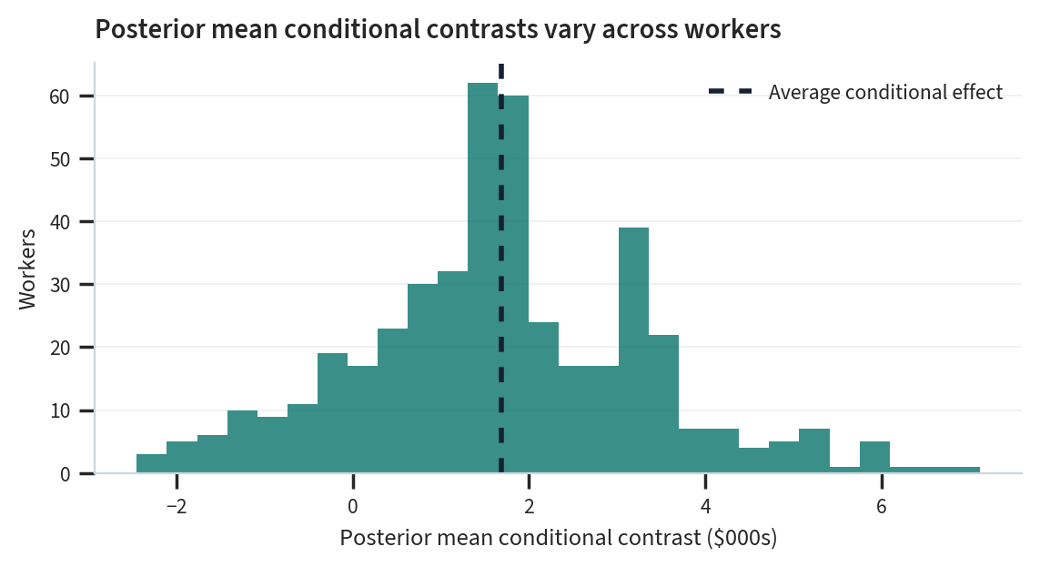
Figure 8: The histogram shows the distribution across workers of posterior mean conditional contrasts under Model 2. The dashed line is their average over the observed workers.

ate_sample_m1 = np.asarray(imputations_m1["tau_sample"])
ate_sample_m2 = np.asarray(imputations_m2["tau_sample"])
ate_comparison_bins = np.histogram_bin_edges(
    np.concatenate([ate_sample_m1, ate_sample_m2]),
    bins=32,
)

fig, ax = plt.subplots(figsize=(5.6, 3.0))
plot_step_histogram(
    ate_sample_m1,
    label="Model 1: no covariates",
    color=COLORS["baseline"],
    bins=ate_comparison_bins,
    ax=ax,
)
plot_step_histogram(
    ate_sample_m2,
    label="Model 2: with covariates",
    color=COLORS["expanded"],
    bins=ate_comparison_bins,
    ax=ax,
)
add_reference_line(ax)
ax.set_xlabel("Finite-sample ATE ($000s)")
ax.set_ylabel("Density")
ax.set_title("Covariates modestly lower the ATE")
ax.legend(title=None)
plt.show()

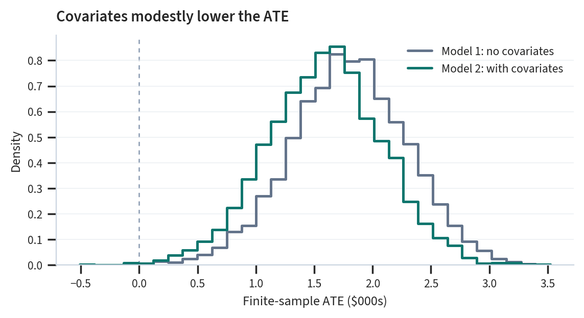
Figure 9: Unsmoothed density histograms compare posterior finite-sample ATE draws under the two Normal models. Both models use the same bin edges; the vertical line marks no average effect.

What covariates repaired, and what they did not

Model 2 can explain systematic differences in conditional means and can express heterogeneous conditional mean effects. The sample-standardized effect \tau^X and the realized finite-sample ATE \tau^S both have posterior means of about $1.6 thousand here. Their numerical agreement is a result, not an identity: the first averages regression contrasts over the observed covariates, while the second averages contrasts from completed potential-outcome schedules.

The posterior predictive diagnosis is more consequential. About 35% of control outcomes and 24% of treated outcomes are exactly zero, while the replicated share is always zero. The model instead puts about 21% of each arm below zero. Replicated skewness is centered near zero, compared with observed skewness of 1.82 in the control arm and 2.72 in the treated arm. Those failures are almost unchanged because they come from the Normal outcome family, not from omitted predictors.

This is the point of the controlled comparison. Covariates may improve prediction and imputation, but they cannot repair impossible support or create a point mass. The next model changes the outcome family in direct response to those predictive failures.

Model 3: a hurdle LogNormal model

Earnings have two scientifically distinct parts: whether a worker has positive earnings and, if so, how much they earn. Let E_i(w) indicate positive earnings under treatment level w. The model is

\begin{aligned} E_i(w)&\sim\operatorname{Bernoulli}(p_w),\\ Y_i(w)\mid E_i(w)=1&\sim\operatorname{LogNormal}(\mu_w,\sigma_w^2),\\ Y_i(w)\mid E_i(w)=0&=0. \end{aligned}

This is a hurdle model, or equivalently a point-mass mixture at zero. I avoid the looser label “zero-inflated” because zero is not in the support of the LogNormal component. The likelihood for one outcome is

p(y\mid p_w,\mu_w,\sigma_w)= \begin{cases} 1-p_w,&y=0,\\ p_w\,\operatorname{LogNormal}(y\mid\mu_w,\sigma_w),&y>0. \end{cases}

During NUTS, the binary positive-earnings indicator is marginalized and the closed-form log likelihood is added with numpyro.factor. This is statistically useful, not merely a coding trick: NUTS cannot sample a discrete latent gate. In prior and posterior predictive simulation, sampling the gate directly is fine.

The priors are calibrated on the original earnings scale through prior predictive checks:

1-p_w\sim\operatorname{Beta}(2,2),\qquad \mu_w\sim\mathcal{N}(1.8,0.75^2),\qquad \sigma_w\sim\operatorname{HalfNormal}(0.75).

The population mean is p_w\exp(\mu_w+\sigma_w^2/2). Population quantiles come from the full mixture: a quantile is zero when its probability level lies inside the point mass, and otherwise it is the appropriately rescaled LogNormal quantile. This matters because subtracting the conditional positive-earnings quantiles would not give the marginal population QTE.

I report the population ATE \tau^{\mathrm{pop}}, its population QTEs, and the corresponding finite-sample estimands from completed schedules. I also report two margin-specific contrasts: p_1-p_0 for the probability of positive earnings and \mathbb{E}\{Y_i(1)\mid Y_i(1)>0\}-\mathbb{E}\{Y_i(0)\mid Y_i(0)>0\}. The contrasts have different units and should not be added together.

The second contrast needs a careful label. It compares treatment-specific groups of positive earners, and those groups need not contain the same workers. It is therefore not a causal effect for a common population. A principal-stratification estimand could instead compare outcomes among workers with positive earnings under both treatments, but that target depends on the joint distribution of the two potential positive-earnings indicators and requires assumptions beyond randomization. I report the marginal contrast because it describes the two-part outcome distribution, not because it answers the principal-stratum question. A future tutorial will take up that principal-stratification problem directly.

The finite-sample intervals below use the conditional cross-world independence implied by the separate control and treatment sampling sites. Other couplings with the same fitted marginals would leave the observed-data fit unchanged but could alter uncertainty in \tau^S and the finite-sample QTEs.

From the mixture to the helper functions

The two hurdle helpers below are direct translations of the mixture distribution. Let g=P(Y=0)=1-p_w be the probability of the zero gate, and let f_{\mathrm{LN}} and F_{\mathrm{LN}} denote the LogNormal density and CDF. After marginalizing the binary indicator, one observation contributes

\log p(y\mid g,\mu,\sigma)= \begin{cases} -\infty,&y<0,\\ \log g,&y=0,\\ \log(1-g)+\log f_{\mathrm{LN}}(y\mid\mu,\sigma),&y>0. \end{cases}

This is the calculation in hurdle_lognormal_logp. For a positive value, the marginal CDF is

F(y)=g+(1-g)F_{\mathrm{LN}}(y).

Hamiltonian Monte Carlo relies on gradients and therefore cannot move directly through discrete latent variables. For NUTS, we marginalize the gate analytically. NumPyro can enumerate some discrete latent variables, but the closed-form marginalization here is simpler and typically more efficient.

Solving F(y)=q gives the marginal quantile

Q(q)= \begin{cases} 0,&q\le g,\\ F_{\mathrm{LN}}^{-1}\!\left(\dfrac{q-g}{1-g}\right),&q>g. \end{cases}

The second helper implements this rescaling. It is what makes the reported population QTEs quantiles of the full point-mass mixture rather than quantiles conditional on positive earnings.³

def hurdle_lognormal_logp(y, gate, mu, sig):
    """Log density after marginalizing E ~ Bernoulli(1 - gate)."""
    safe_y = jnp.where(y > 0, y, jnp.ones_like(y))
    log_p_zero = jnp.log(gate)
    log_p_positive = (
        jnp.log1p(-gate) + dist.LogNormal(mu, sig).log_prob(safe_y)
    )
    return jnp.where(
        y == 0, log_p_zero, jnp.where(y > 0, log_p_positive, -jnp.inf)
    )


assert np.isneginf(
    np.asarray(hurdle_lognormal_logp(jnp.array([-1.0]), 0.5, 0.0, 1.0))[0]
)


def hurdle_lognormal_quantile(q, gate, mu, sig):
    """Marginal quantile of a point mass at zero plus a LogNormal."""
    positive_probability = 1 - gate
    q_positive = jnp.clip(
        (q - gate) / positive_probability, 1e-6, 1 - 1e-6
    )
    positive_quantile = dist.LogNormal(mu, sig).icdf(q_positive)
    return jnp.where(q <= gate, 0.0, positive_quantile)


def positive_quantile_draws(y_rep, q):
    return np.array(
        [
            np.quantile(row[row > 0], q) if np.any(row > 0) else np.nan
            for row in y_rep
        ]
    )


def model3(df, mode="fit"):
    valid_modes = ("fit", "replicate", "impute")
    if mode not in valid_modes:
        raise ValueError(f"`mode` must be one of {valid_modes}, got {mode!r}.")

    N = df.shape[0]
    w = jnp.asarray(df["treat"].to_numpy(), dtype=bool)
    y = jnp.asarray(df["re78"].to_numpy())
    q = jnp.array([0.25, 0.50, 0.75])

    gate_0 = numpyro.sample("gate_0", dist.Beta(2, 2))
    gate_1 = numpyro.sample("gate_1", dist.Beta(2, 2))
    mu_0 = numpyro.sample("mu_0", dist.Normal(1.8, 0.75))
    mu_1 = numpyro.sample("mu_1", dist.Normal(1.8, 0.75))
    sig_0 = numpyro.sample("sig_0", dist.HalfNormal(0.75))
    sig_1 = numpyro.sample("sig_1", dist.HalfNormal(0.75))

    p_positive_0 = 1 - gate_0
    p_positive_1 = 1 - gate_1
    mean_positive_0 = jnp.exp(mu_0 + sig_0**2 / 2)
    mean_positive_1 = jnp.exp(mu_1 + sig_1**2 / 2)

    if mode == "fit":
        logp_0 = hurdle_lognormal_logp(y, gate_0, mu_0, sig_0)
        logp_1 = hurdle_lognormal_logp(y, gate_1, mu_1, sig_1)
        with numpyro.plate("unit", N):
            numpyro.factor("lik_y0", jnp.where(~w, logp_0, 0.0))
            numpyro.factor("lik_y1", jnp.where(w, logp_1, 0.0))

    if mode != "fit":
        numpyro.deterministic(
            "tau_pop",
            p_positive_1 * mean_positive_1
            - p_positive_0 * mean_positive_0,
        )
        numpyro.deterministic(
            "tau_qte_pop",
            hurdle_lognormal_quantile(q, gate_1, mu_1, sig_1)
            - hurdle_lognormal_quantile(q, gate_0, mu_0, sig_0),
        )
        numpyro.deterministic(
            "delta_p_positive", p_positive_1 - p_positive_0
        )
        numpyro.deterministic(
            "delta_mean_positive", mean_positive_1 - mean_positive_0
        )

        with numpyro.plate("unit", N):
            e_0 = numpyro.sample("e_0", dist.Bernoulli(p_positive_0))
            e_1 = numpyro.sample("e_1", dist.Bernoulli(p_positive_1))
            y_0_positive = numpyro.sample(
                "y_0_positive", dist.LogNormal(mu_0, sig_0)
            )
            y_1_positive = numpyro.sample(
                "y_1_positive", dist.LogNormal(mu_1, sig_1)
            )
            y_0 = jnp.where(e_0 == 1, y_0_positive, 0.0)
            y_1 = jnp.where(e_1 == 1, y_1_positive, 0.0)

    if mode == "replicate":
        numpyro.deterministic("y_rep", jnp.where(w, y_1, y_0))

    if mode == "impute":
        y_0_imp = numpyro.deterministic(
            "y_0_imp", jnp.where(w, y_0, y)
        )
        y_1_imp = numpyro.deterministic(
            "y_1_imp", jnp.where(w, y, y_1)
        )
        numpyro.deterministic(
            "tau_sample", jnp.mean(y_1_imp - y_0_imp)
        )
        numpyro.deterministic(
            "tau_qte_sample",
            jnp.quantile(y_1_imp, q) - jnp.quantile(y_0_imp, q),
        )

def hurdle_ppc_statistic_table(y_obs, y_rep, arm):
    y_obs_positive = y_obs[y_obs > 0]
    statistics = {
        "Share equal to zero": (
            np.mean(y_obs == 0),
            np.mean(y_rep == 0, axis=1),
        ),
        "Median positive earnings": (
            np.median(y_obs_positive),
            positive_quantile_draws(y_rep, 0.50),
        ),
        "90th percentile, positive earnings": (
            np.quantile(y_obs_positive, 0.90),
            positive_quantile_draws(y_rep, 0.90),
        ),
        "95th percentile, positive earnings": (
            np.quantile(y_obs_positive, 0.95),
            positive_quantile_draws(y_rep, 0.95),
        ),
    }
    return pl.DataFrame(
        [
            {
                "arm": arm,
                "statistic": name,
                "observed": observed,
                "predictive_median": np.nanmedian(draws),
                "predictive_05": np.nanquantile(draws, 0.05),
                "predictive_95": np.nanquantile(draws, 0.95),
            }
            for name, (observed, draws) in statistics.items()
        ]
    )


def summarize_named_draws(samples, labels):
    return pl.DataFrame(
        [
            {
                "estimand": label,
                "mean": np.mean(draws),
                "sd": np.std(draws),
                "p05": np.quantile(draws, 0.05),
                "p50": np.quantile(draws, 0.50),
                "p95": np.quantile(draws, 0.95),
            }
            for name, label in labels.items()
            for draws in [np.asarray(samples[name])]
        ]
    )

Prior predictive checks

The prior predictive check evaluates the two parts of the science separately. For each arm, I compare the zero share and the median, 90th percentile, and 95th percentile among positive earners. I also inspect the population ATE, the marginal population QTEs, and the two margin-specific contrasts.

key, prior_key_m3 = jr.split(key)
prior_predictive_m3 = infer.Predictive(
    model3,
    num_samples=500,
    return_sites=[
        "y_rep", "tau_pop", "tau_qte_pop",
        "delta_p_positive", "delta_mean_positive",
    ],
)
prior_samples_m3 = prior_predictive_m3(
    prior_key_m3, df=df, mode="replicate"
)

w_m3 = df["treat"].to_numpy().astype(bool)
y_m3 = df["re78"].to_numpy()
y_prior_m3 = np.asarray(prior_samples_m3["y_rep"])
prior_checks_m3 = pl.concat(
    [
        hurdle_ppc_statistic_table(
            y_m3[~w_m3], y_prior_m3[:, ~w_m3], "Control"
        ),
        hurdle_ppc_statistic_table(
            y_m3[w_m3], y_prior_m3[:, w_m3], "Treated"
        ),
    ]
)
display(
    prior_checks_m3.style.fmt_number(
        columns=[
            "observed", "predictive_median", "predictive_05",
            "predictive_95",
        ],
        decimals=2,
    )
)

arm	statistic	observed	predictive_median	predictive_05	predictive_95
Control	Share equal to zero	0.35	0.52	0.13	0.86
Control	Median positive earnings	5.77	6.09	1.83	22.12
Control	90th percentile, positive earnings	13.89	12.68	3.03	75.89
Control	95th percentile, positive earnings	16.82	15.24	3.21	118.67
Treated	Share equal to zero	0.24	0.48	0.14	0.87
Treated	Median positive earnings	6.50	6.27	1.74	23.26
Treated	90th percentile, positive earnings	17.28	11.90	3.07	68.19
Treated	95th percentile, positive earnings	22.21	14.36	3.34	105.31

prior_effects_m3 = {
    "tau_pop": np.asarray(prior_samples_m3["tau_pop"]),
    "tau_q25_pop": np.asarray(prior_samples_m3["tau_qte_pop"])[:, 0],
    "tau_q50_pop": np.asarray(prior_samples_m3["tau_qte_pop"])[:, 1],
    "tau_q75_pop": np.asarray(prior_samples_m3["tau_qte_pop"])[:, 2],
    "delta_p_positive": np.asarray(
        prior_samples_m3["delta_p_positive"]
    ),
    "delta_mean_positive": np.asarray(
        prior_samples_m3["delta_mean_positive"]
    ),
}
prior_effect_labels_m3 = {
    "tau_pop": r"Population ATE $\tau^{\mathrm{pop}}$",
    "tau_q25_pop": "Population QTE, 25th percentile",
    "tau_q50_pop": "Population QTE, median",
    "tau_q75_pop": "Population QTE, 75th percentile",
    "delta_p_positive": "Change in probability of positive earnings",
    "delta_mean_positive": "Positive-earnings conditional contrast",
}
display(
    summarize_named_draws(
        prior_effects_m3, prior_effect_labels_m3
    ).style.fmt_number(
        columns=["mean", "sd", "p05", "p50", "p95"], decimals=2
    )
)

estimand	mean	sd	p05	p50	p95
Population ATE $\tau^{\mathrm{pop}}$	0.53	13.62	−14.58	0.35	14.40
Population QTE, 25th percentile	−0.11	3.84	−4.37	0.00	4.35
Population QTE, median	0.53	7.39	−9.87	0.00	13.06
Population QTE, 75th percentile	0.60	12.56	−17.71	0.51	19.08
Change in probability of positive earnings	0.02	0.33	−0.54	0.03	0.55
Positive-earnings conditional contrast	0.34	22.79	−26.82	0.35	25.71

Unlike the Normal models, every prior predictive outcome is nonnegative and exact zeros occur with positive probability. The observed arm-level summaries fall inside the displayed prior predictive intervals. The treatment contrasts have medians near zero, while the positive-earnings distributions remain broad enough to cover the observed upper tails. On these dimensions, the prior predictive distribution is much better matched to the application.

Fitting the observed-data model

In fit mode, the gate is marginalized and numpyro.factor adds the closed-form hurdle likelihood for the observed treatment arm. NUTS therefore samples only the six continuous parameters. In replicate and impute modes, sampling the binary positive-earnings indicators is valid because those calls run outside NUTS.

key, fit_key_m3 = jr.split(key)
sampler_m3 = infer.MCMC(
    infer.NUTS(model3, target_accept_prob=0.90),
    num_samples=1_000,
    num_warmup=1_000,
    num_chains=4,
    chain_method="sequential",
    progress_bar=False,
)
sampler_m3.run(fit_key_m3, df=df, mode="fit")
# sampler_m3.print_summary(exclude_deterministic=True)

posterior_samples_m3 = sampler_m3.get_samples()
m3_idata = az.from_numpyro(sampler_m3)
az.summary(
    m3_idata,
    var_names=["gate_0", "gate_1", "mu_0", "mu_1", "sig_0", "sig_1"],
)

	mean	sd	eti89_lb	eti89_ub	ess_bulk	ess_tail	r_hat	mcse_mean	mcse_sd
gate_0	0.3559	0.0294	0.31	0.4	5919	3035	1.00	0.00038	0.00028
gate_1	0.2485	0.0312	0.2	0.3	6028	2533	1.00	0.0004	0.00029
mu_0	1.599	0.077	1.5	1.7	7061	3194	1.00	0.00092	0.00064
mu_1	1.69	0.084	1.6	1.8	6383	3060	1.00	0.0011	0.00075
sig_0	1.004	0.056	0.92	1.1	5935	3294	1.00	0.00073	0.00052
sig_1	1.037	0.062	0.94	1.1	6469	3151	1.00	0.00078	0.00056

Posterior predictive checks and causal imputation

The four NUTS chains completed without divergences, and the reported \widehat R values round to 1.00. I now call the fitted model twice. Replication asks whether the hurdle model reproduces the zero shares and the distribution of positive earnings in each arm. Imputation combines observed factual outcomes with simulated counterfactuals and produces completed potential-outcome schedules. Keeping the calls separate prevents a replicated observed dataset from being mistaken for a causal completion.

key, ppc_key_m3, imputation_key_m3 = jr.split(key, 3)

posterior_predictive_m3 = infer.Predictive(
    model3,
    posterior_samples=posterior_samples_m3,
    return_sites=[
        "y_rep", "tau_pop", "tau_qte_pop",
        "delta_p_positive", "delta_mean_positive",
    ],
)
ppc_m3 = posterior_predictive_m3(
    ppc_key_m3, df=df, mode="replicate"
)
y_rep_m3 = np.asarray(ppc_m3["y_rep"])
ppc_summary_m3 = pl.concat(
    [
        hurdle_ppc_statistic_table(
            y_m3[~w_m3], y_rep_m3[:, ~w_m3], "Control"
        ),
        hurdle_ppc_statistic_table(
            y_m3[w_m3], y_rep_m3[:, w_m3], "Treated"
        ),
    ]
)
display(
    ppc_summary_m3.style.fmt_number(
        columns=[
            "observed", "predictive_median", "predictive_05",
            "predictive_95",
        ],
        decimals=2,
    )
)

posterior_imputation_m3 = infer.Predictive(
    model3,
    posterior_samples=posterior_samples_m3,
    return_sites=[
        "y_0_imp", "y_1_imp", "tau_pop", "tau_qte_pop",
        "tau_sample", "tau_qte_sample",
        "delta_p_positive", "delta_mean_positive",
    ],
)
imputations_m3 = posterior_imputation_m3(
    imputation_key_m3, df=df, mode="impute"
)

arm	statistic	observed	predictive_median	predictive_05	predictive_95
Control	Share equal to zero	0.35	0.36	0.29	0.42
Control	Median positive earnings	5.77	4.95	4.04	6.07
Control	90th percentile, positive earnings	13.89	17.61	13.60	23.47
Control	95th percentile, positive earnings	16.82	24.93	18.45	35.52
Treated	Share equal to zero	0.24	0.25	0.18	0.32
Treated	Median positive earnings	6.50	5.42	4.29	6.81
Treated	90th percentile, positive earnings	17.28	19.97	14.96	27.88
Treated	95th percentile, positive earnings	22.21	28.54	20.29	42.17

effects_m3 = {
    "tau_pop": np.asarray(imputations_m3["tau_pop"]),
    "tau_sample": np.asarray(imputations_m3["tau_sample"]),
    "tau_q25_pop": np.asarray(imputations_m3["tau_qte_pop"])[:, 0],
    "tau_q50_pop": np.asarray(imputations_m3["tau_qte_pop"])[:, 1],
    "tau_q75_pop": np.asarray(imputations_m3["tau_qte_pop"])[:, 2],
    "tau_q25_sample": np.asarray(
        imputations_m3["tau_qte_sample"]
    )[:, 0],
    "tau_q50_sample": np.asarray(
        imputations_m3["tau_qte_sample"]
    )[:, 1],
    "tau_q75_sample": np.asarray(
        imputations_m3["tau_qte_sample"]
    )[:, 2],
    "delta_p_positive": np.asarray(
        imputations_m3["delta_p_positive"]
    ),
    "delta_mean_positive": np.asarray(
        imputations_m3["delta_mean_positive"]
    ),
}
effect_labels_m3 = {
    "tau_pop": r"Population ATE $\tau^{\mathrm{pop}}$",
    "tau_sample": r"Finite-sample ATE $\tau^S$",
    "tau_q25_pop": "Population QTE, 25th percentile",
    "tau_q50_pop": "Population QTE, median",
    "tau_q75_pop": "Population QTE, 75th percentile",
    "tau_q25_sample": "Finite-sample QTE, 25th percentile",
    "tau_q50_sample": "Finite-sample QTE, median",
    "tau_q75_sample": "Finite-sample QTE, 75th percentile",
    "delta_p_positive": "Change in probability of positive earnings",
    "delta_mean_positive": "Positive-earnings conditional contrast",
}
effects_summary_m3 = summarize_named_draws(
    effects_m3, effect_labels_m3
)
display(
    effects_summary_m3.style.fmt_number(
        columns=["mean", "sd", "p05", "p50", "p95"], decimals=2
    )
)

estimand	mean	sd	p05	p50	p95
Population ATE $\tau^{\mathrm{pop}}$	1.72	1.01	0.17	1.68	3.43
Finite-sample ATE $\tau^S$	1.88	0.75	0.72	1.83	3.13
Population QTE, 25th percentile	0.40	0.43	0.00	0.31	1.16
Population QTE, median	1.18	0.55	0.29	1.17	2.09
Population QTE, 75th percentile	1.92	1.05	0.27	1.88	3.71
Finite-sample QTE, 25th percentile	0.36	0.34	0.00	0.39	0.93
Finite-sample QTE, median	1.17	0.52	0.28	1.18	2.00
Finite-sample QTE, 75th percentile	1.95	0.72	0.83	1.97	3.06
Change in probability of positive earnings	0.11	0.04	0.04	0.11	0.18
Positive-earnings conditional contrast	1.11	1.29	−0.91	1.06	3.27

# hide-code-pdf-source: paired-with-cell-class
fig_control_m3, ax_control_m3 = plt.subplots(figsize=(3.1, 2.5))
fig_treated_m3, ax_treated_m3 = plt.subplots(figsize=(3.1, 2.5))
plot_posterior_predictive_by_arm(
    y_m3,
    y_rep_m3[:100],
    w_m3,
    axes=(ax_control_m3, ax_treated_m3),
    positive=True,
    title="The upper tail remains too heavy",
)
plt.show()

(a) Control.

(b) Treated.

Figure 10: Black lines show observed positive-earnings ECDFs; teal lines and mint bands show posterior predictive medians and central 80% envelopes across 100 Model 3 replications.

What Model 3 repaired

Model 3 directly repairs the failures that covariates could not. Replicated earnings are never negative, exact zeros have positive probability, and the positive outcomes can be right-skewed. The zero shares are reproduced closely: the posterior predictive medians are 0.358 for controls and 0.249 for treated units, compared with observed shares of 0.354 and 0.243.

The positive-earnings medians are somewhat low, and the upper tail remains too heavy. The predictive medians of the positive-earnings 95th percentile are 24.9 and 28.5, compared with observed values of 16.8 and 22.2. The hurdle fixes the impossible support and zero mass, but the simple arm-level LogNormal component does not completely reproduce the earnings tail.

The posterior mean of the population ATE \tau^{\mathrm{pop}} is 1.72, with a central 90% interval from 0.17 to 3.43. The finite-sample ATE \tau^S has posterior mean 1.88 and a central 90% interval from 0.72 to 3.13. These estimands describe different targets, so their numerical similarity is a result rather than an identity.

The average probability of positive earnings increases by 0.107, with a central 90% interval from 0.037 to 0.177. The positive-earnings conditional contrast is 1.11, with a central 90% interval from -0.91 to 3.27. The clearer signal is on the extensive margin, while the conditional contrast remains uncertain and does not describe an effect for a common positive-earner population.

Model 3 still assigns the same hurdle probability and positive-earnings distribution to every unit in a treatment arm. Model 4 keeps the repaired outcome family and asks whether pre-treatment covariates explain systematic variation in both margins.

Model 4: let both hurdle components depend on covariates

Model 3 gives every unit in an arm the same probability of positive earnings and the same distribution of earnings among workers. The final model lets both parts vary with the pre-treatment covariates \mathbf{X}_i. For w\in\{0,1\},

\begin{aligned} E_i(w)\mid\mathbf{X}_i,\theta &\sim\operatorname{Bernoulli}\!\left(p_{iw}\right),\\ \operatorname{logit}(p_{iw}) &=\alpha_{pw}+\mathbf{X}_i^\top\gamma_w,\\ \log Y_i(w)\mid E_i(w)=1,\mathbf{X}_i,\theta &\sim\mathcal{N}\!\left(\alpha_{\mu w}+\mathbf{X}_i^\top\beta_w,\sigma_w^2\right),\\ Y_i(w)\mid E_i(w)=0&=0. \end{aligned}

The employment component describes the extensive margin. The positive-earnings component describes the intensive margin. Treatment can shift either component, and the model does not force the same covariate relationships in the two treatment arms.

I reuse the nine-column design matrix from Model 2: standardized age, educ, re74, and re75, followed by the binary indicators black, married, nodegr, u74, and u75. This matches the nine covariate rows in Table 8.7 of Imbens and Rubin, in addition to an intercept. hisp is available in the data but is not part of that specification.

The priors are weakly informative on the scales created by this design matrix. A broader first pass put too much prior mass on enormous earnings because the LogNormal transformation amplifies uncertainty on the log scale. The scales below retain substantial uncertainty while keeping the prior predictive outcomes in a useful range:

\begin{aligned} \alpha_{pw}&\sim\mathcal{N}(0,1^2), & \gamma_{wk}&\sim\mathcal{N}(0,0.5^2),\\ \alpha_{\mu w}&\sim\mathcal{N}(1.8,0.75^2), & \beta_{wk}&\sim\mathcal{N}(0,0.25^2), & \sigma_w&\sim\operatorname{HalfNormal}(0.75). \end{aligned}

For each observed covariate profile, the model-implied conditional mean is

m_{iw}=p_{iw}\exp\!\left(\alpha_{\mu w}+\mathbf{X}_i^\top\beta_w+\frac{\sigma_w^2}{2}\right).

The contrast m_{i1}-m_{i0} is a conditional mean treatment effect, not a realized individual effect. I call its average over the observed covariate profiles \tau^X. The realized finite-sample ATE \tau^S still comes from completed potential-outcome schedules. I also report two sample-standardized component contrasts: the difference in positive-earnings probabilities and the difference between treatment-specific means conditional on positive earnings. These contrasts have different units and are not an additive decomposition of \tau^X; the second also compares treatment-specific conditioning groups, not a common population.

Prior predictive checks

Before fitting, I check the implied zero shares, the scale and upper tail of positive earnings, and the three treatment-effect summaries. This is especially important for a LogNormal regression because modest changes on the log scale can produce very large earnings on the original scale. The observed arm-level summaries fall inside the displayed prior predictive intervals, while the treatment-effect priors remain centered near zero.

def model4(w, y, X, mode="fit", subsample_size=None):
    valid_modes = ("fit", "replicate", "impute")
    if mode not in valid_modes:
        raise ValueError(f"`mode` must be one of {valid_modes}, got {mode!r}.")

    w = jnp.asarray(w, dtype=bool)
    y = jnp.asarray(y)
    X = jnp.asarray(X)
    if w.ndim != 1 or y.ndim != 1 or X.ndim != 2:
        raise ValueError("`w` and `y` must be 1D and `X` must be 2D.")
    N, K = X.shape
    if w.shape[0] != N or y.shape[0] != N:
        raise ValueError("`w`, `y`, and the rows of `X` must align.")
    if mode != "fit" and subsample_size is not None:
        raise ValueError("Subsampling is available only when `mode='fit'`.")

    alpha_pos_0 = numpyro.sample("alpha_pos_0", dist.Normal(0, 1))
    alpha_pos_1 = numpyro.sample("alpha_pos_1", dist.Normal(0, 1))
    gamma_0 = numpyro.sample("gamma_0", dist.Normal(0, 0.5).expand([K]))
    gamma_1 = numpyro.sample("gamma_1", dist.Normal(0, 0.5).expand([K]))

    alpha_mu_0 = numpyro.sample("alpha_mu_0", dist.Normal(1.8, 0.75))
    alpha_mu_1 = numpyro.sample("alpha_mu_1", dist.Normal(1.8, 0.75))
    beta_0 = numpyro.sample("beta_0", dist.Normal(0, 0.25).expand([K]))
    beta_1 = numpyro.sample("beta_1", dist.Normal(0, 0.25).expand([K]))
    sig_0 = numpyro.sample("sig_0", dist.HalfNormal(0.75))
    sig_1 = numpyro.sample("sig_1", dist.HalfNormal(0.75))

    if mode == "fit":
        with numpyro.plate("unit", N, subsample_size=subsample_size) as idx:
            w_batch, y_batch, X_batch = w[idx], y[idx], X[idx]
            p_pos_0 = jax.nn.sigmoid(alpha_pos_0 + X_batch @ gamma_0)
            p_pos_1 = jax.nn.sigmoid(alpha_pos_1 + X_batch @ gamma_1)
            mu_0 = alpha_mu_0 + X_batch @ beta_0
            mu_1 = alpha_mu_1 + X_batch @ beta_1
            lp_0 = hurdle_lognormal_logp(
                y_batch, 1 - p_pos_0, mu_0, sig_0
            )
            lp_1 = hurdle_lognormal_logp(
                y_batch, 1 - p_pos_1, mu_1, sig_1
            )
            numpyro.factor("lik_y0", jnp.where(~w_batch, lp_0, 0.0))
            numpyro.factor("lik_y1", jnp.where(w_batch, lp_1, 0.0))
        return

    p_pos_0 = jax.nn.sigmoid(alpha_pos_0 + X @ gamma_0)
    p_pos_1 = jax.nn.sigmoid(alpha_pos_1 + X @ gamma_1)
    mu_0 = alpha_mu_0 + X @ beta_0
    mu_1 = alpha_mu_1 + X @ beta_1

    with numpyro.plate("unit", N):
        employed_0 = numpyro.sample("employed_0", dist.Bernoulli(p_pos_0))
        employed_1 = numpyro.sample("employed_1", dist.Bernoulli(p_pos_1))
        y_0_positive = numpyro.sample(
            "y_0_positive", dist.LogNormal(mu_0, sig_0)
        )
        y_1_positive = numpyro.sample(
            "y_1_positive", dist.LogNormal(mu_1, sig_1)
        )
        y_0 = numpyro.deterministic(
            "y_0", jnp.where(employed_0.astype(bool), y_0_positive, 0.0)
        )
        y_1 = numpyro.deterministic(
            "y_1", jnp.where(employed_1.astype(bool), y_1_positive, 0.0)
        )

    mean_positive_0 = jnp.exp(mu_0 + sig_0**2 / 2)
    mean_positive_1 = jnp.exp(mu_1 + sig_1**2 / 2)
    mean_outcome_0 = p_pos_0 * mean_positive_0
    mean_outcome_1 = p_pos_1 * mean_positive_1
    tau_cond = numpyro.deterministic(
        "tau_cond", mean_outcome_1 - mean_outcome_0
    )
    numpyro.deterministic("tau_x", jnp.mean(tau_cond))
    numpyro.deterministic(
        "delta_p_positive", jnp.mean(p_pos_1 - p_pos_0)
    )
    numpyro.deterministic(
        "delta_mean_positive", jnp.mean(mean_positive_1 - mean_positive_0)
    )

    if mode == "replicate":
        numpyro.deterministic("y_rep", jnp.where(w, y_1, y_0))

    if mode == "impute":
        q = jnp.array([0.25, 0.50, 0.75])
        y_0_imp = numpyro.deterministic("y_0_imp", jnp.where(w, y_0, y))
        y_1_imp = numpyro.deterministic("y_1_imp", jnp.where(w, y, y_1))
        numpyro.deterministic(
            "tau_sample", jnp.mean(y_1_imp - y_0_imp)
        )
        numpyro.deterministic(
            "tau_qte_sample",
            jnp.quantile(y_1_imp, q) - jnp.quantile(y_0_imp, q),
        )

w_m4 = df["treat"].to_numpy().astype(bool)
y_m4 = df["re78"].to_numpy()
key, prior_key_m4 = jr.split(key)
prior_predictive_m4 = infer.Predictive(
    model4,
    num_samples=500,
    return_sites=[
        "y_rep", "tau_x", "delta_p_positive", "delta_mean_positive"
    ],
)
prior_samples_m4 = prior_predictive_m4(
    prior_key_m4, w=w_m4, y=y_m4, X=X, mode="replicate"
)
y_prior_m4 = np.asarray(prior_samples_m4["y_rep"])
prior_checks_m4 = pl.concat(
    [
        hurdle_ppc_statistic_table(
            y_m4[~w_m4], y_prior_m4[:, ~w_m4], "Control"
        ),
        hurdle_ppc_statistic_table(
            y_m4[w_m4], y_prior_m4[:, w_m4], "Treated"
        ),
    ]
)
display(
    prior_checks_m4.style.fmt_number(
        columns=[
            "observed", "predictive_median", "predictive_05", "predictive_95"
        ],
        decimals=2,
    )
)

prior_effect_labels_m4 = {
    "tau_x": r"Sample-standardized mean effect $\tau^X$",
    "delta_p_positive": "Change in probability of positive earnings",
    "delta_mean_positive": "Positive-earnings conditional contrast",
}
display(
    summarize_named_draws(
        prior_samples_m4, prior_effect_labels_m4
    ).style.fmt_number(
        columns=["mean", "sd", "p05", "p50", "p95"], decimals=2
    )
)

arm	statistic	observed	predictive_median	predictive_05	predictive_95
Control	Share equal to zero	0.35	0.48	0.14	0.85
Control	Median positive earnings	5.77	5.50	1.39	27.78
Control	90th percentile, positive earnings	13.89	14.35	3.59	91.42
Control	95th percentile, positive earnings	16.82	19.93	4.24	156.37
Treated	Share equal to zero	0.24	0.52	0.15	0.84
Treated	Median positive earnings	6.50	6.30	1.45	28.84
Treated	90th percentile, positive earnings	17.28	16.69	3.23	97.99
Treated	95th percentile, positive earnings	22.21	21.24	4.19	146.10

estimand	mean	sd	p05	p50	p95
Sample-standardized mean effect $\tau^X$	−0.15	18.86	−22.84	0.18	23.72
Change in probability of positive earnings	−0.02	0.32	−0.54	−0.02	0.51
Positive-earnings conditional contrast	1.09	37.08	−37.63	0.54	42.05

Fitting the observed-data model

As in Model 3, fitting marginalizes the discrete positive-earnings indicators and evaluates the hurdle likelihood with numpyro.factor. NUTS therefore samples only continuous parameters. The predictive modes sample those indicators directly because they run outside NUTS. The appendix in Section 7.2 uses the same model interface with minibatches and stochastic variational inference when a full-data NUTS fit is no longer practical.

key, fit_key_m4 = jr.split(key)
sampler_m4 = infer.MCMC(
    infer.NUTS(model4, target_accept_prob=0.90),
    num_samples=1_000,
    num_warmup=1_000,
    num_chains=4,
    chain_method="sequential",
    progress_bar=False,
)
sampler_m4.run(fit_key_m4, w=w_m4, y=y_m4, X=X, mode="fit")
# sampler_m4.print_summary(exclude_deterministic=True)
posterior_samples_m4 = sampler_m4.get_samples()

m4_idata = az.from_numpyro(
    sampler_m4,
    coords={"covariate": x_names},
    dims={
        "beta_0": ["covariate"],
        "beta_1": ["covariate"],
        "gamma_0": ["covariate"],
        "gamma_1": ["covariate"],
    },
)
az.summary(
    m4_idata,
    var_names=[
        "alpha_pos_0", "alpha_pos_1", "gamma_0", "gamma_1",
        "alpha_mu_0", "alpha_mu_1", "beta_0", "beta_1",
        "sig_0", "sig_1",
    ],
)

	mean	sd	eti89_lb	eti89_ub	ess_bulk	ess_tail	r_hat	mcse_mean	mcse_sd
alpha_pos_0	1.19	0.433	0.51	1.9	5097	3239	1.00	0.0061	0.0042
alpha_pos_1	1.35	0.471	0.59	2.1	5092	3106	1.00	0.0066	0.0047
gamma_0[age]	-0.094	0.13	-0.3	0.11	7650	2874	1.00	0.0015	0.001
gamma_0[educ]	-0.046	0.162	-0.3	0.21	6033	3562	1.00	0.0021	0.0015
gamma_0[re74]	0.146	0.194	-0.15	0.47	5581	3049	1.00	0.0026	0.0019
gamma_0[re75]	0.014	0.202	-0.3	0.34	5797	3341	1.00	0.0027	0.0019
gamma_0[black]	-0.564	0.294	-1	-0.096	6141	3207	1.00	0.0038	0.0026
gamma_0[married]	-0.114	0.31	-0.6	0.39	7240	2910	1.00	0.0036	0.0026
gamma_0[nodegr]	-0.029	0.312	-0.53	0.46	5465	3311	1.00	0.0042	0.003
gamma_0[u74]	-0.332	0.344	-0.89	0.21	6113	2958	1.00	0.0044	0.0031
gamma_0[u75]	0.26	0.308	-0.22	0.74	6106	2961	1.00	0.0039	0.0028
gamma_1[age]	0.079	0.175	-0.21	0.36	8052	2821	1.00	0.0019	0.0014
gamma_1[educ]	0.055	0.176	-0.24	0.33	6118	3241	1.00	0.0023	0.0016
gamma_1[re74]	-0.058	0.262	-0.46	0.37	6746	2948	1.00	0.0032	0.0024
gamma_1[re75]	0.434	0.284	-0.0044	0.91	5845	3380	1.00	0.0038	0.0026
gamma_1[black]	-0.472	0.351	-1	0.091	6549	3112	1.00	0.0043	0.0031
gamma_1[married]	0.336	0.357	-0.23	0.91	7063	3245	1.00	0.0042	0.0029
gamma_1[nodegr]	-0.08	0.358	-0.65	0.5	5098	3115	1.00	0.005	0.0035
gamma_1[u74]	0.514	0.376	-0.094	1.1	6840	3016	1.00	0.0045	0.0031
gamma_1[u75]	-0.238	0.377	-0.84	0.35	6317	2841	1.00	0.0048	0.0033
alpha_mu_0	1.92	0.225	1.6	2.3	4489	3177	1.00	0.0034	0.0023
alpha_mu_1	1.685	0.235	1.3	2.1	4502	2981	1.00	0.0035	0.0025
beta_0[age]	0.097	0.075	-0.022	0.22	7178	3333	1.00	0.00088	0.00062
beta_0[educ]	0.005	0.092	-0.14	0.15	5864	3213	1.00	0.0012	0.00085
beta_0[re74]	-0.031	0.088	-0.17	0.11	5563	2855	1.00	0.0012	0.00084
beta_0[re75]	0.053	0.097	-0.1	0.21	5302	3137	1.00	0.0013	0.00096
beta_0[black]	-0.27	0.151	-0.51	-0.029	7202	2994	1.00	0.0018	0.0012
beta_0[married]	-0.114	0.17	-0.39	0.16	6603	3319	1.00	0.0021	0.0015
beta_0[nodegr]	-0.017	0.179	-0.31	0.27	5554	2932	1.00	0.0024	0.0017
beta_0[u74]	-0.083	0.177	-0.37	0.2	5999	3266	1.00	0.0023	0.0016
beta_0[u75]	-0.015	0.173	-0.29	0.27	6223	2931	1.00	0.0022	0.0015
beta_1[age]	-0.001	0.088	-0.14	0.14	5988	3288	1.00	0.0011	0.00082
beta_1[educ]	0.073	0.083	-0.061	0.21	5210	3352	1.00	0.0012	0.00082
beta_1[re74]	-0.029	0.115	-0.21	0.16	6031	3264	1.00	0.0015	0.001
beta_1[re75]	0.067	0.102	-0.096	0.23	6004	3388	1.00	0.0013	0.00096
beta_1[black]	-0.044	0.166	-0.3	0.22	6250	3012	1.00	0.0021	0.0015
beta_1[married]	0.066	0.171	-0.21	0.34	7231	3209	1.00	0.002	0.0015
beta_1[nodegr]	-0.113	0.177	-0.39	0.17	4930	3381	1.00	0.0025	0.0017
beta_1[u74]	0.139	0.195	-0.17	0.45	6261	3111	1.00	0.0025	0.0017
beta_1[u75]	-0.014	0.168	-0.28	0.25	6581	3299	1.00	0.0021	0.0015
sig_0	1	0.0553	0.92	1.1	6956	2950	1.00	0.00067	0.00046
sig_1	1.045	0.064	0.95	1.2	8000	3021	1.00	0.00073	0.00053

Posterior predictive checks and causal imputation

The four NUTS chains completed without divergences. I again keep replication and imputation separate. Replicated observed datasets test whether the fitted model reproduces the arm-specific zero shares and positive-earnings distributions. Completed potential-outcome schedules answer the causal questions only after that model check.

key, ppc_key_m4, imputation_key_m4 = jr.split(key, 3)

posterior_predictive_m4 = infer.Predictive(
    model4,
    posterior_samples=posterior_samples_m4,
    return_sites=[
        "y_rep", "tau_cond", "tau_x",
        "delta_p_positive", "delta_mean_positive",
    ],
)
ppc_m4 = posterior_predictive_m4(
    ppc_key_m4, w=w_m4, y=y_m4, X=X, mode="replicate"
)
y_rep_m4 = np.asarray(ppc_m4["y_rep"])
ppc_summary_m4 = pl.concat(
    [
        hurdle_ppc_statistic_table(
            y_m4[~w_m4], y_rep_m4[:, ~w_m4], "Control"
        ),
        hurdle_ppc_statistic_table(
            y_m4[w_m4], y_rep_m4[:, w_m4], "Treated"
        ),
    ]
)
display(
    ppc_summary_m4.style.fmt_number(
        columns=[
            "observed", "predictive_median", "predictive_05", "predictive_95"
        ],
        decimals=2,
    )
)

posterior_imputation_m4 = infer.Predictive(
    model4,
    posterior_samples=posterior_samples_m4,
    return_sites=[
        "y_0_imp", "y_1_imp", "tau_cond", "tau_x",
        "delta_p_positive", "delta_mean_positive",
        "tau_sample", "tau_qte_sample",
    ],
)
imputations_m4 = posterior_imputation_m4(
    imputation_key_m4, w=w_m4, y=y_m4, X=X, mode="impute"
)

effects_m4 = {
    "tau_x": np.asarray(imputations_m4["tau_x"]),
    "tau_sample": np.asarray(imputations_m4["tau_sample"]),
    "tau_q25_sample": np.asarray(imputations_m4["tau_qte_sample"])[:, 0],
    "tau_q50_sample": np.asarray(imputations_m4["tau_qte_sample"])[:, 1],
    "tau_q75_sample": np.asarray(imputations_m4["tau_qte_sample"])[:, 2],
    "delta_p_positive": np.asarray(imputations_m4["delta_p_positive"]),
    "delta_mean_positive": np.asarray(
        imputations_m4["delta_mean_positive"]
    ),
}
effect_labels_m4 = {
    "tau_x": r"Sample-standardized mean effect $\tau^X$",
    "tau_sample": r"Finite-sample ATE $\tau^S$",
    "tau_q25_sample": "Finite-sample QTE, 25th percentile",
    "tau_q50_sample": "Finite-sample QTE, median",
    "tau_q75_sample": "Finite-sample QTE, 75th percentile",
    "delta_p_positive": "Change in probability of positive earnings",
    "delta_mean_positive": "Positive-earnings conditional contrast",
}
display(
    summarize_named_draws(
        effects_m4, effect_labels_m4
    ).style.fmt_number(
        columns=["mean", "sd", "p05", "p50", "p95"], decimals=2
    )
)

arm	statistic	observed	predictive_median	predictive_05	predictive_95
Control	Share equal to zero	0.35	0.36	0.29	0.43
Control	Median positive earnings	5.77	4.90	4.01	6.03
Control	90th percentile, positive earnings	13.89	17.97	13.80	24.01
Control	95th percentile, positive earnings	16.82	25.71	18.91	36.34
Treated	Share equal to zero	0.24	0.25	0.18	0.32
Treated	Median positive earnings	6.50	5.41	4.25	6.81
Treated	90th percentile, positive earnings	17.28	20.91	15.37	29.24
Treated	95th percentile, positive earnings	22.21	30.29	21.02	45.22

estimand	mean	sd	p05	p50	p95
Sample-standardized mean effect $\tau^X$	1.68	1.06	0.00	1.62	3.47
Finite-sample ATE $\tau^S$	1.78	0.78	0.55	1.74	3.13
Finite-sample QTE, 25th percentile	0.26	0.31	0.00	0.00	0.76
Finite-sample QTE, median	1.06	0.54	0.17	1.07	1.93
Finite-sample QTE, 75th percentile	1.81	0.74	0.67	1.78	3.01
Change in probability of positive earnings	0.10	0.04	0.03	0.10	0.17
Positive-earnings conditional contrast	1.05	1.41	−1.22	1.00	3.47

# hide-code-pdf-source: paired-with-cell-class
fig_control_m4, ax_control_m4 = plt.subplots(figsize=(3.1, 2.5))
fig_treated_m4, ax_treated_m4 = plt.subplots(figsize=(3.1, 2.5))
plot_posterior_predictive_by_arm(
    y_m4,
    y_rep_m4[:100],
    w_m4,
    axes=(ax_control_m4, ax_treated_m4),
    positive=True,
    title="Covariates do not repair the tail",
)
plt.show()

(a) Control.

(b) Treated.

Figure 11: Black lines show observed positive-earnings ECDFs; teal lines and mint bands show posterior predictive medians and central 80% envelopes across 100 Model 4 replications.

tau_cond_m4 = np.asarray(imputations_m4["tau_cond"])
fig, ax = plt.subplots(figsize=(5.6, 3.0))
posterior_mean_tau_cond_m4 = tau_cond_m4.mean(axis=0)
plot_effect_heterogeneity(posterior_mean_tau_cond_m4, ax=ax)
ax.set_xlabel("Posterior mean conditional contrast ($000s)")
ax.set_ylabel("Workers")
ax.set_title("Posterior mean conditional contrasts vary across workers")
ax.legend(title=None)
plt.show()

Figure 12: The histogram shows the distribution across workers of posterior mean conditional contrasts under Model 4. The dashed line is their average over the observed workers.

What Model 4 adds

Model 4 preserves the support repair from Model 3 while allowing the extensive and intensive margins to vary systematically with pre-treatment characteristics. The posterior predictive checks therefore have two jobs: verify that the hurdle still reproduces zeros and positive-earnings tails, and check whether the additional regression structure has improved those predictions rather than merely producing more coefficients.

The zero shares are reproduced closely: the posterior predictive medians are 0.358 for controls and 0.249 for treated units, compared with observed shares of 0.354 and 0.243. The positive-earnings medians are somewhat low, and the upper tail remains too heavy. For example, the predictive medians of the positive-earnings 95th percentile are 25.7 and 30.3, compared with observed values of 16.8 and 22.2. The hurdle solves the support problem, but the LogNormal component still leaves a visible tail mismatch.

The posterior mean of the sample-standardized conditional mean effect \tau^X is 1.68, with a central 90% interval from 0.00 to 3.47. The finite-sample ATE \tau^S, based on completed potential-outcome schedules, has posterior mean 1.78 and a central 90% interval from 0.55 to 3.13. The average probability of positive earnings increases by 0.104, with a central 90% interval from 0.031 to 0.172. The positive-earnings conditional contrast is 1.05, with a central 90% interval from -1.22 to 3.47. The clearer signal is on the extensive margin; the conditional contrast remains uncertain and does not describe an effect for a common positive-earner population.

The vector tau_cond contains conditional mean contrasts m_{i1}-m_{i0} for the observed covariate profiles. It does not contain realized individual treatment effects. The latter still require a joint potential-outcome schedule and remain unidentified for every unit.

Posterior parameter table: a Table 8.7 analogue

Table 8.7 in Imbens and Rubin reports the control-arm coefficients and the treated-minus-control differences for the positive-earnings coefficients \beta and the employment coefficients \gamma. The table below follows that layout. Entries are posterior means with posterior standard deviations in parentheses.

This is an analogue rather than a direct reproduction for three reasons:

1. age, educ, re74, and re75 are standardized here, while the book uses their raw scales.
2. The priors here are weakly informative and chosen through prior predictive reasoning, while Chapter 8 describes its priors only as diffuse.
3. The comparison checks parameter ordering, units, transformations, and signs; it does not use numerical agreement as the organizing goal.

Both implementations model P(Y(w)>0\mid X) directly, so the employment coefficients have the same sign convention.

ps = posterior_samples_m4

beta_0_s   = np.array(ps["beta_0"])        # (S, K)
beta_1_s   = np.array(ps["beta_1"])
gamma_0_s  = np.array(ps["gamma_0"])
gamma_1_s  = np.array(ps["gamma_1"])
a_mu_0_s   = np.array(ps["alpha_mu_0"])    # (S,)
a_mu_1_s   = np.array(ps["alpha_mu_1"])
a_pos_0_s   = np.array(ps["alpha_pos_0"])
a_pos_1_s   = np.array(ps["alpha_pos_1"])
sig_0_s    = np.array(ps["sig_0"])
sig_1_s    = np.array(ps["sig_1"])

def ms(arr):
    if arr is None:
        return ""
    return f"{np.mean(arr):.2f} ({np.std(arr):.2f})"

def make_row(cov, bc_arr, dbc_arr, g0_arr, dg_arr):
    return {
        "covariate": cov,
        "beta_c": ms(bc_arr),
        "beta_t - beta_c": ms(dbc_arr),
        "gamma_0": ms(g0_arr),
        "gamma_1 - gamma_0": ms(dg_arr),
    }

rows = [make_row(
    "intercept",
    a_mu_0_s,          a_mu_1_s   - a_mu_0_s,
    a_pos_0_s,         a_pos_1_s - a_pos_0_s,
)]
for j, name in enumerate(x_names):
    rows.append(make_row(
        name,
        beta_0_s[:, j],  (beta_1_s  - beta_0_s)[:, j],
        gamma_0_s[:, j], (gamma_1_s - gamma_0_s)[:, j],
    ))
rows.append(make_row("ln(sigma_c)", np.log(sig_0_s), None, None, None))
rows.append(make_row("ln(sigma_t)", np.log(sig_1_s), None, None, None))

tbl87 = pl.DataFrame(rows)
(
    tbl87.style
    .cols_label(
        cases={
            "beta_c": "beta_c (SD)",
            "beta_t - beta_c": "beta diff. (SD)",
            "gamma_0": "gamma_0 (SD)",
            "gamma_1 - gamma_0": "gamma diff. (SD)",
        }
    )
    .tab_options(table_width="100%", table_font_size="8px")
)

covariate	beta_c (SD)	beta diff. (SD)	gamma_0 (SD)	gamma diff. (SD)
intercept	1.92 (0.22)	-0.24 (0.32)	1.19 (0.43)	0.15 (0.64)
age	0.10 (0.07)	-0.10 (0.12)	-0.09 (0.13)	0.17 (0.22)
educ	0.01 (0.09)	0.07 (0.12)	-0.05 (0.16)	0.10 (0.24)
re74	-0.03 (0.09)	0.00 (0.14)	0.15 (0.19)	-0.20 (0.33)
re75	0.05 (0.10)	0.01 (0.14)	0.01 (0.20)	0.42 (0.34)
black	-0.27 (0.15)	0.23 (0.22)	-0.56 (0.29)	0.09 (0.45)
married	-0.11 (0.17)	0.18 (0.24)	-0.11 (0.31)	0.45 (0.47)
nodegr	-0.02 (0.18)	-0.10 (0.25)	-0.03 (0.31)	-0.05 (0.48)
u74	-0.08 (0.18)	0.22 (0.26)	-0.33 (0.34)	0.85 (0.52)
u75	-0.02 (0.17)	0.00 (0.24)	0.26 (0.31)	-0.50 (0.50)
ln(sigma_c)	-0.00 (0.06)
ln(sigma_t)	0.04 (0.06)

Comparing the four models

The table below compares the same causal estimand across all four models: the finite-sample ATE \tau^S calculated from completed potential-outcome schedules. The posterior predictive verdict is a separate assessment of whether each fitted model can reproduce important features of the observed earnings data. Similar causal estimates do not imply similar predictive fit.

comparison_specs = [
    {
        "model": "Model 1",
        "outcome_family": "Normal",
        "covariates": "No",
        "imputations": imputations_m1,
        "verdict": (
            "Fails: negatives, no zeros, symmetric."
        ),
    },
    {
        "model": "Model 2",
        "outcome_family": "Normal",
        "covariates": "Yes",
        "imputations": imputations_m2,
        "verdict": (
            "Covariates do not repair those failures."
        ),
    },
    {
        "model": "Model 3",
        "outcome_family": "Hurdle LogNormal",
        "covariates": "No",
        "imputations": imputations_m3,
        "verdict": (
            "Support fixed; positive tail too heavy."
        ),
    },
    {
        "model": "Model 4",
        "outcome_family": "Hurdle LogNormal",
        "covariates": "Yes",
        "imputations": imputations_m4,
        "verdict": (
            "Covariates added; positive tail heavy."
        ),
    },
]

comparison_rows = []
for spec in comparison_specs:
    tau_sample_draws = np.asarray(spec["imputations"]["tau_sample"])
    assert tau_sample_draws.ndim == 1
    p05, p95 = np.quantile(tau_sample_draws, [0.05, 0.95])
    comparison_rows.append(
        {
            "Model": spec["model"],
            "Outcome family": spec["outcome_family"],
            "Covariates": spec["covariates"],
            "Finite-sample ATE mean": np.mean(tau_sample_draws),
            "Central 90% interval": f"[{p05:.2f}, {p95:.2f}]",
            "Posterior predictive verdict": spec["verdict"],
        }
    )

model_comparison = pl.DataFrame(comparison_rows)
(
    model_comparison.style.fmt_number(
        columns=["Finite-sample ATE mean"], decimals=2
    )
    .cols_label(
        cases={
            "Finite-sample ATE mean": "ATE mean",
            "Central 90% interval": "Central 90%",
            "Posterior predictive verdict": "PPC verdict",
        }
    )
    .cols_width(
        cases={
            "Model": "70px",
            "Outcome family": "110px",
            "Covariates": "65px",
            "Finite-sample ATE mean": "80px",
            "Central 90% interval": "100px",
            "Posterior predictive verdict": "260px",
        }
    )
    .tab_options(table_width="100%", table_font_size="8px")
)

Table 1: A common finite-sample estimand and posterior predictive verdict across the four models.

Model	Outcome family	Covariates	ATE mean	Central 90%	PPC verdict
Model 1	Normal	No	1.80	[0.97, 2.61]	Fails: negatives, no zeros, symmetric.
Model 2	Normal	Yes	1.59	[0.78, 2.39]	Covariates do not repair those failures.
Model 3	Hurdle LogNormal	No	1.88	[0.72, 3.13]	Support fixed; positive tail too heavy.
Model 4	Hurdle LogNormal	Yes	1.78	[0.55, 3.13]	Covariates added; positive tail heavy.

The sequence matters more than the final row. Model 1 establishes a useful baseline, but its Normal outcome family generates negative earnings, cannot generate exact zeros, and misses the strong right skew. Model 2 shows what changes when we add pre-treatment covariates while holding that outcome family fixed. The covariates describe conditional means and heterogeneity, but they cannot repair a likelihood with the wrong support and shape.

Model 3 changes the outcome family in direct response to those failures. Its hurdle separates the probability of positive earnings from the amount earned when earnings are positive. This removes negative outcomes, reproduces the point mass at zero, and allows right skew. The remaining positive-earnings upper tail is still too heavy. Model 4 then lets covariates enter both hurdle components. It adds systematic heterogeneity while preserving the support repair, but the tail mismatch does not disappear.

The finite-sample ATE is fairly stable across these models. That stability is a robustness observation about this estimand, not a posterior predictive check and not evidence that the Normal models fit the outcome distribution. In both hurdle models, the clearer signal is an increase in the probability of positive earnings. The positive-earnings conditional contrast remains uncertain and does not describe a causal effect for a common population.

Finally, conditional mean contrasts such as m_{i1}-m_{i0} are not realized individual treatment effects. A realized effect requires both potential outcomes for the same unit. Completing those schedules depends on an unidentified joint potential-outcome distribution. The sensitivity appendix illustrates that dependence using Model 1.

Conclusion: where Model 4 leaves us

Model 4 is a useful pedagogical stopping point, with qualifications. It repairs the outcome support, represents exact zeros and right skew, and lets pre-treatment covariates shape both the extensive and intensive margins. The checks in Figure 11 also show why it is not an unqualified winner: its positive-earnings distribution still places too much mass in the upper tail.

The stability of the finite-sample ATE across Table 1 is reassuring for that estimand. Under Model 4 its posterior mean is about 1.8 thousand, with a central 90% interval from about 0.6 to 3.1 thousand. The clearest component signal is the average increase of about 0.10 in the probability of positive earnings. The positive-earnings conditional contrast remains uncertain. Stable ATEs do not validate every causal summary: tail-sensitive estimands, including finite-sample QTEs, remain sensitive to the outcome family.

Individual effects and probabilities of benefit require the joint distribution of the two potential outcomes, not just their fitted marginal distributions. That cross-world dependence is not identified by the observed data (Ding and Li 2018; Mealli et al. 2023). The Model 1 appendix exercise shows the same issue for posterior uncertainty in a finite-sample estimand: changing \rho alters the completed schedules even though the observed-data fit is unchanged.

The most complex model is not automatically the best model. Following the iterative Bayesian workflow of Gelman et al. (2020), the reusable lesson is to keep the scientific question, model criticism, and causal imputation in the right order:

1. Define the science and the assignment mechanism.
2. Fit only the observed-data likelihood.
3. Check replicated observed data against the features that matter scientifically.
4. Repair predictive failures with scientifically motivated structure, changing one assumption at a time when possible.
5. Impute missing potential outcomes only after checking the fitted model.
6. Report each estimand with its target population and identifying assumptions.

The immediate controlled revision would be a hurdle Gamma regression: keep the two-part structure and covariate specification, but replace the LogNormal positive-earnings component and ask whether the upper-tail check improves. If a Gamma distribution is still too restrictive, a generalized Gamma or a mixture model would be the next candidate. Each revision should go through the same prior predictive checks, computational diagnostics, posterior predictive checks, and estimand and sensitivity comparisons rather than being accepted because it is more flexible.

Beyond that model revision, the next steps are to examine prior sensitivity, carry the cross-world sensitivity analysis into the richer hurdle model, use out-of-sample predictive evaluation when it serves the scientific question, and connect the posterior causal summaries to an explicit policy decision with costs and utilities. When data size makes full MCMC impractical, the SVI scaling appendix shows how stochastic variational inference can scale the same model structure, with an explicit tradeoff in posterior fidelity.

Model 4 is where this tutorial stops, not where the workflow ends.

Appendix

Sensitivity to dependence between potential outcomes

The theory section on potential-outcome dependence explains why the observed-data likelihood identifies the marginal outcome parameters but not the association between Y_i(0) and Y_i(1). Model 1 makes the resulting sensitivity especially transparent because its bivariate Normal Science uses a single association parameter,

\rho=\operatorname{Corr}\!\left\{Y_i(0),Y_i(1)\mid\theta^m\right\}.

The main Model 1 analysis fixes \rho=0. Here I leave its fitted marginal distributions unchanged, fix \rho at three illustrative values, and repeat only the causal-imputation step using Equation 8. This is a sensitivity analysis, not an attempt to estimate \rho. Under the independent prior parameterization described in the theory section, placing a prior on \rho would simply pass that prior into the posterior.

This limitation is not repaired by moving to a more flexible likelihood. Model 1 is used here because the correlation is easy to interpret; richer marginal models still require assumptions about how the two potential outcomes are paired for the same worker.

def rho_sensitivity_samples(posterior_samples, df, rho, rng_key):
    w = df["treat"].to_numpy().astype(bool)
    y = jnp.asarray(df["re78"].to_numpy())
    q = jnp.array([0.25, 0.50, 0.75])
    mu_0 = jnp.asarray(posterior_samples["mu_0"])
    mu_1 = jnp.asarray(posterior_samples["mu_1"])
    sig_0 = jnp.asarray(posterior_samples["sig_0"])
    sig_1 = jnp.asarray(posterior_samples["sig_1"])
    n_draws = mu_0.shape[0]
    n_units = y.shape[0]
    eps0, eps1 = jr.normal(rng_key, (2, n_draws, n_units))
    cond_sd0 = sig_0 * jnp.sqrt(1 - rho**2)
    cond_sd1 = sig_1 * jnp.sqrt(1 - rho**2)
    y0_mis = (
        mu_0[:, None]
        + rho * (sig_0 / sig_1)[:, None] * (y[None, :] - mu_1[:, None])
        + cond_sd0[:, None] * eps0
    )
    y1_mis = (
        mu_1[:, None]
        + rho * (sig_1 / sig_0)[:, None] * (y[None, :] - mu_0[:, None])
        + cond_sd1[:, None] * eps1
    )
    y0_imp = jnp.where(w[None, :], y0_mis, y[None, :])
    y1_imp = jnp.where(w[None, :], y[None, :], y1_mis)
    qte = jnp.quantile(y1_imp, q, axis=1) - jnp.quantile(y0_imp, q, axis=1)
    return {
        "rho": np.repeat(rho, n_draws),
        "tau_sample": np.asarray(jnp.mean(y1_imp - y0_imp, axis=1)),
        "tau_q25_sample": np.asarray(qte[0]),
        "tau_q50_sample": np.asarray(qte[1]),
        "tau_q75_sample": np.asarray(qte[2]),
    }

rho_values = [-0.5, 0.0, 0.5]
rho_key = jr.PRNGKey(20260801)
rho_sensitivity = [
    rho_sensitivity_samples(
        posterior_samples_m1, df, rho, jr.fold_in(rho_key, i)
    )
    for i, rho in enumerate(rho_values)
]
rho_sensitivity_df = pl.concat(
    [pl.DataFrame(draws) for draws in rho_sensitivity]
)
rho_summary = (
    rho_sensitivity_df
    .group_by("rho")
    .agg(
        pl.col("tau_sample").mean().alias("tau_sample_mean"),
        pl.col("tau_sample").std().alias("tau_sample_sd"),
        pl.col("tau_q25_sample").quantile(0.05).alias("tau_q25_05"),
        pl.col("tau_q25_sample").quantile(0.95).alias("tau_q25_95"),
        pl.col("tau_q50_sample").quantile(0.05).alias("tau_q50_05"),
        pl.col("tau_q50_sample").quantile(0.95).alias("tau_q50_95"),
        pl.col("tau_q75_sample").quantile(0.05).alias("tau_q75_05"),
        pl.col("tau_q75_sample").quantile(0.95).alias("tau_q75_95"),
    )
    .sort("rho")
)

rho_summary_compact = rho_summary.select(
    pl.col("rho").alias("Correlation"),
    pl.col("tau_sample_mean").alias("ATE mean"),
    pl.col("tau_sample_sd").alias("ATE SD"),
    pl.concat_str(
        pl.lit("["), pl.col("tau_q25_05").round(2), pl.lit(", "),
        pl.col("tau_q25_95").round(2), pl.lit("]"),
    ).alias("QTE 25%"),
    pl.concat_str(
        pl.lit("["), pl.col("tau_q50_05").round(2), pl.lit(", "),
        pl.col("tau_q50_95").round(2), pl.lit("]"),
    ).alias("QTE 50%"),
    pl.concat_str(
        pl.lit("["), pl.col("tau_q75_05").round(2), pl.lit(", "),
        pl.col("tau_q75_95").round(2), pl.lit("]"),
    ).alias("QTE 75%"),
)
rho_summary_compact.style.fmt_number(
    columns=["Correlation", "ATE mean", "ATE SD"], decimals=2
)

Table 2: Model 1 sensitivity to the fixed potential-outcome correlation. Earnings are measured in thousands of dollars; QTE entries are central 90% intervals.

Correlation	ATE mean	ATE SD	QTE 25%	QTE 50%	QTE 75%
−0.50	1.79	0.39	[0.0, 1.29]	[0.95, 2.47]	[2.19, 4.03]
0.00	1.79	0.51	[0.0, 1.19]	[0.73, 2.61]	[2.03, 4.17]
0.50	1.79	0.59	[0.0, 1.24]	[0.54, 2.67]	[1.89, 4.16]

The posterior mean of the finite-sample ATE remains close to 1.79 across Table 2, but its posterior standard deviation increases with \rho in this application. The finite-sample QTE intervals also change because every value of \rho implies a different way of completing the same 445 potential-outcome pairs. There is no general monotonicity result for arbitrary finite-sample estimands: \rho changes both the conditional means and conditional variances of the missing outcomes.

By contrast, the population ATE and the population QTEs are functions of the fitted marginal distributions and remain unchanged. The sensitivity shown here is a consequence of the causal target and the missing joint information, not a computational failure.

fig, ax = plt.subplots(figsize=(6.2, 2.3))
ax.plot(
    rho_summary.get_column("rho").to_numpy(),
    rho_summary.get_column("tau_sample_sd").to_numpy(),
    color=COLORS["posterior"],
    linewidth=2.5,
    marker="o",
    markersize=6.5,
)
ax.set(
    xlabel="Fixed correlation",
    ylabel="Posterior SD of finite-sample ATE ($000s)",
    title="Correlation assumptions change uncertainty",
)
ax.set_xticks(rho_summary.get_column("rho").to_numpy())
ax.tick_params(colors=COLORS["muted"])
ax.xaxis.label.set_color(COLORS["muted"])
ax.yaxis.label.set_color(COLORS["muted"])
ax.title.set_color(COLORS["ink"])
plt.show()

Figure 13: The observed-data likelihood is unchanged across the three fixed correlations. Only the completion of the missing potential outcomes changes.

Scaling Model 4 with stochastic variational inference

When it is computationally feasible, NUTS is a useful reference method because it generates correlated draws that target the specified posterior rather than restricting inference to a chosen approximation family. Diagnostics such as divergences, \widehat R, and effective sample size can reveal sampling problems, but clean diagnostics do not prove that the statistical model is well specified. Its computational cost can grow quickly with the number of observations and gradient evaluations.

SVI takes a different route: it turns posterior inference into an optimization problem. We choose a tractable family q_\phi(\theta), called the guide, and tune its parameters \phi to approximate the posterior p(\theta\mid y). The guide is a computational approximation, not a second model for the data. Here AutoNormal uses a mean-field guide: after mapping constrained parameters to an unconstrained space, it represents the latent components with independent Normal factors. This is inexpensive, but it cannot represent posterior correlations and may distort marginal uncertainty.

The objective is the evidence lower bound,

\operatorname{ELBO}(\phi)=\mathbb{E}_{q_\phi(\theta)}\!\left[\log p(y,\theta)-\log q_\phi(\theta)\right]=\log p(y)-\operatorname{KL}\!\left\{q_\phi(\theta)\,\|\,p(\theta\mid y)\right\}.

Because \log p(y) does not depend on \phi, maximizing the ELBO is equivalent to minimizing this KL divergence within the chosen guide family. NumPyro reports a stochastic estimate of the negative ELBO, which the optimizer minimizes. Here that estimate uses one guide draw and a fresh minibatch at each step, so the raw trace is expected to be noisy. For a statistical introduction, see Blei et al. (2017); the official NumPyro SVI documentation covers the API.

A loss trace that falls and stabilizes supports a narrow conclusion: the optimizer has reached a stable region of the chosen objective. It does not show that the optimizer found the global optimum, that the guide is flexible enough, or that posterior means and intervals are accurate. Recovery against known simulation truth, repeated fits from different seeds, posterior predictive checks, and comparison with NUTS on a manageable subset probe those separate questions.

To make scale and recovery observable rather than asserted, I simulate 100,000 workers from Model 4. The four continuous covariates are standard Normal and the five indicators have probabilities 0.45, 0.35, 0.65, 0.40, and 0.35. Treatment is randomized with probability one half. The data seed is fixed, and the true parameters below are deliberately on the same standardized scale as the tutorial’s design matrix.

N_SVI = 100_000
DATA_SEED_SVI = 20260731
OPTIMIZATION_SEED_SVI = 20260732
POSTERIOR_SEED_SVI = 20260733
COMPARISON_SEED_SVI = 20260734

rng_svi = np.random.default_rng(DATA_SEED_SVI)
X_cont_svi = rng_svi.normal(size=(N_SVI, 4))
binary_prob_svi = np.array([0.45, 0.35, 0.65, 0.40, 0.35])
X_binary_svi = rng_svi.binomial(1, binary_prob_svi, size=(N_SVI, 5))
X_svi = np.column_stack([X_cont_svi, X_binary_svi]).astype(np.float32)
w_svi = rng_svi.binomial(1, 0.5, size=N_SVI).astype(bool)

alpha_pos_true_svi = np.array([0.35, 0.75], dtype=np.float32)
gamma_true_svi = np.array(
    [
        [0.18, 0.12, 0.10, 0.15, -0.25, 0.20, -0.18, -0.25, -0.20],
        [0.23, 0.12, 0.06, 0.18, -0.20, 0.18, -0.14, -0.23, -0.19],
    ],
    dtype=np.float32,
)
alpha_mu_true_svi = np.array([1.75, 1.90], dtype=np.float32)
beta_true_svi = np.array(
    [
        [0.08, 0.06, 0.12, 0.10, -0.08, 0.07, -0.06, -0.10, -0.08],
        [0.10, 0.07, 0.11, 0.12, -0.06, 0.06, -0.05, -0.10, -0.07],
    ],
    dtype=np.float32,
)
sig_true_svi = np.array([0.55, 0.60], dtype=np.float32)

logit_pos_svi = alpha_pos_true_svi[:, None] + gamma_true_svi @ X_svi.T
p_pos_true_svi = jax.nn.sigmoid(jnp.asarray(logit_pos_svi))
mu_true_svi = alpha_mu_true_svi[:, None] + beta_true_svi @ X_svi.T
p_observed_svi = np.asarray(
    jnp.where(jnp.asarray(w_svi), p_pos_true_svi[1], p_pos_true_svi[0])
)
mu_observed_svi = np.where(w_svi, mu_true_svi[1], mu_true_svi[0])
sig_observed_svi = np.where(w_svi, sig_true_svi[1], sig_true_svi[0])
employed_svi = rng_svi.binomial(1, p_observed_svi).astype(bool)
positive_y_svi = rng_svi.lognormal(mu_observed_svi, sig_observed_svi)
y_svi = np.where(employed_svi, positive_y_svi, 0.0).astype(np.float32)

mean_positive_true_svi = np.exp(
    mu_true_svi + sig_true_svi[:, None] ** 2 / 2
)
mean_outcome_true_svi = np.asarray(p_pos_true_svi) * mean_positive_true_svi
true_estimands_svi = {
    "tau_x": np.mean(mean_outcome_true_svi[1] - mean_outcome_true_svi[0]),
    "delta_p_positive": np.mean(
        np.asarray(p_pos_true_svi[1] - p_pos_true_svi[0])
    ),
    "delta_mean_positive": np.mean(
        mean_positive_true_svi[1] - mean_positive_true_svi[0]
    ),
}

The subsample_size argument added to model4 changes only fitting. Inside numpyro.plate, NumPyro selects 2,048 rows and automatically scales their log likelihood to represent all 100,000 observations; there is no manual likelihood multiplier. Replication and imputation continue to use every row and reject subsampling.

I optimize the one-particle ELBO for 6,000 steps. The clipped Adam learning rate starts at 10^{-2} and halves every 2,000 steps.

Table 3: Large-data SVI configuration. The fit reports its current runtime below; that number includes JAX compilation and is not a hardware-independent benchmark.

Configuration	Value
Data and minibatches	100,000 rows; 2,048-row minibatches
Optimization	6,000 steps; one-particle ELBO; 122.88 effective data passes
Guide	AutoNormal mean-field approximation
Optimizer	Clipped Adam; initial rate 10^{-2}; 2,000-step half-decay
Posterior summaries	1,000 guide draws evaluated in chunks of 50
Seeds	20260731 data; 20260732 optimization; 20260733 guide draws

Hardware, precision, software versions, the guide, and the geometry of a new dataset can all change runtime materially.

SVI_BATCH_SIZE = 2_048
SVI_STEPS = 6_000
SVI_DRAWS = 1_000
SVI_DRAW_CHUNK = 50

guide_svi = AutoNormal(
    model4, init_loc_fn=init_to_median(num_samples=10)
)
learning_rate_svi = exponential_decay(
    1e-2, decay_steps=2_000, decay_rate=0.5
)
optimizer_svi = numpyro.optim.ClippedAdam(
    learning_rate_svi, clip_norm=10.0
)
svi = infer.SVI(
    model4,
    guide_svi,
    optimizer_svi,
    loss=infer.Trace_ELBO(num_particles=1),
)

svi_start = time.perf_counter()
svi_result = svi.run(
    jr.PRNGKey(OPTIMIZATION_SEED_SVI),
    SVI_STEPS,
    w=w_svi,
    y=y_svi,
    X=X_svi,
    mode="fit",
    subsample_size=SVI_BATCH_SIZE,
    progress_bar=False,
)
jax.block_until_ready(svi_result.losses)
svi_runtime_seconds = time.perf_counter() - svi_start
svi_loss_per_observation = np.asarray(svi_result.losses) / N_SVI
print(
    f"SVI fit, including JAX compilation: "
    f"{svi_runtime_seconds:.1f} seconds on CPU"
)

SVI fit, including JAX compilation: 24.7 seconds on CPU

smooth_window_svi = 101
smooth_loss_svi = np.convolve(
    svi_loss_per_observation,
    np.ones(smooth_window_svi) / smooth_window_svi,
    mode="valid",
)
smooth_steps_svi = np.arange(
    smooth_window_svi // 2 + 1,
    SVI_STEPS - smooth_window_svi // 2 + 1,
)

fig, ax = plt.subplots(figsize=(6.2, 3.2))
ax.plot(
    np.arange(1, SVI_STEPS + 1),
    svi_loss_per_observation,
    color=COLORS["reference"],
    linewidth=0.6,
    alpha=0.35,
    label="Raw minibatch loss",
)
ax.plot(
    smooth_steps_svi,
    smooth_loss_svi,
    color=COLORS["posterior"],
    linewidth=2.0,
    label="101-step moving average",
)
ax.set(
    xlabel="Optimization step",
    ylabel="Negative ELBO per observation",
    title="The stochastic objective stabilizes",
)
ax.legend(title=None)
plt.show()

Figure 14: The raw negative ELBO per observation is noisy because each update uses a fresh minibatch. The 101-step moving average falls rapidly and then stabilizes, diagnosing optimization but not posterior accuracy.

The convergence trace in Figure 14 is an optimization diagnostic: it shows that the stochastic objective has stabilized. It does not establish that the variational family accurately represents the posterior. Approximation quality is a separate question, addressed in the optional approximation checks.

For posterior draw s, define the fitted probability of positive earnings and the fitted mean among positive earners as

p_{iw}^{(s)}=\operatorname{logit}^{-1}\!\left(\alpha_{w,\mathrm{pos}}^{(s)}+\mathbf{X}_i^\top\gamma_w^{(s)}\right), \qquad m_{iw,+}^{(s)}=\exp\!\left(\alpha_{w,\mu}^{(s)}+\mathbf{X}_i^\top\beta_w^{(s)}+\frac{(\sigma_w^{(s)})^2}{2}\right).

The implementation reports three sample-standardized contrasts for every draw:

\tau^{X,(s)}=\frac{1}{N}\sum_{i=1}^N\left\{p_{i1}^{(s)}m_{i1,+}^{(s)}-p_{i0}^{(s)}m_{i0,+}^{(s)}\right\},

\Delta_p^{(s)}=\frac{1}{N}\sum_{i=1}^N\left\{p_{i1}^{(s)}-p_{i0}^{(s)}\right\}, \qquad \Delta_+^{(s)}=\frac{1}{N}\sum_{i=1}^N\left\{m_{i1,+}^{(s)}-m_{i0,+}^{(s)}\right\}.

Materializing the fitted values for all S=1{,}000 posterior draws and all N=100{,}000 workers would require intermediate arrays with memory proportional to O(SN). Instead, the code evaluates C=50 draws at a time, immediately averages over workers, and discards the unit-level values before moving to the next chunk. Peak intermediate memory is therefore O(CN), while the retained result has only 3S entries—one value of each estimand for every posterior draw. Chunking changes the memory footprint, not the estimands.

@jax.jit
def model4_estimand_chunk(params, X_eval):
    p_0 = jax.nn.sigmoid(
        params["alpha_pos_0"][:, None] + params["gamma_0"] @ X_eval.T
    )
    p_1 = jax.nn.sigmoid(
        params["alpha_pos_1"][:, None] + params["gamma_1"] @ X_eval.T
    )
    mu_0 = params["alpha_mu_0"][:, None] + params["beta_0"] @ X_eval.T
    mu_1 = params["alpha_mu_1"][:, None] + params["beta_1"] @ X_eval.T
    mean_positive_0 = jnp.exp(mu_0 + params["sig_0"][:, None] ** 2 / 2)
    mean_positive_1 = jnp.exp(mu_1 + params["sig_1"][:, None] ** 2 / 2)
    return jnp.column_stack(
        [
            jnp.mean(
                p_1 * mean_positive_1 - p_0 * mean_positive_0, axis=1
            ),
            jnp.mean(p_1 - p_0, axis=1),
            jnp.mean(mean_positive_1 - mean_positive_0, axis=1),
        ]
    )


def model4_estimands(posterior_samples, X_eval, chunk_size=50):
    n_draws = np.asarray(posterior_samples["alpha_pos_0"]).shape[0]
    chunks = []
    for start in range(0, n_draws, chunk_size):
        stop = min(start + chunk_size, n_draws)
        params_chunk = jt.map(
            lambda value: jnp.asarray(value[start:stop]), posterior_samples
        )
        chunks.append(
            np.asarray(model4_estimand_chunk(params_chunk, jnp.asarray(X_eval)))
        )
    values = np.concatenate(chunks, axis=0)
    return {
        "tau_x": values[:, 0],
        "delta_p_positive": values[:, 1],
        "delta_mean_positive": values[:, 2],
    }


posterior_samples_svi = guide_svi.sample_posterior(
    jr.PRNGKey(POSTERIOR_SEED_SVI),
    svi_result.params,
    sample_shape=(SVI_DRAWS,),
)
estimands_svi = model4_estimands(
    posterior_samples_svi, X_svi, chunk_size=SVI_DRAW_CHUNK
)

Checking the SVI approximation

The scaling walkthrough establishes that the optimization ran and shows how to compute the target summaries without materializing every unit-by-draw prediction. It does not establish posterior fidelity. This optional section checks the approximation in two complementary ways: recovery against the known simulation truth, and comparison with NUTS on a subset small enough for MCMC. The checking code is available in folded blocks on the website; the results remain visible in both formats.

Recovery against simulation truth

assert np.isfinite(svi_loss_per_observation).all()
assert (
    svi_loss_per_observation[-250:].mean()
    < svi_loss_per_observation[:250].mean()
)

estimand_labels_svi = {
    "tau_x": "Sample-standardized mean effect (tau^X)",
    "delta_p_positive": "Change in probability of positive earnings",
    "delta_mean_positive": "Positive-earnings conditional contrast",
}
recovery_rows_svi = []
for name, label in estimand_labels_svi.items():
    draws = estimands_svi[name]
    truth = float(true_estimands_svi[name])
    lower, upper = np.quantile(draws, [0.05, 0.95])
    recovery_rows_svi.append(
        {
            "Estimand": label,
            "Truth": truth,
            "SVI mean": np.mean(draws),
            "Absolute error": abs(np.mean(draws) - truth),
            "Central 90% interval": f"[{lower:.3f}, {upper:.3f}]",
            "Covers truth": bool(lower <= truth <= upper),
        }
    )

recovery_errors_svi = {
    row["Estimand"]: row["Absolute error"] for row in recovery_rows_svi
}
assert recovery_errors_svi[estimand_labels_svi["tau_x"]] <= 0.20
assert (
    recovery_errors_svi[estimand_labels_svi["delta_p_positive"]] <= 0.02
)
assert (
    recovery_errors_svi[estimand_labels_svi["delta_mean_positive"]]
    <= 0.25
)

svi_recovery = pl.DataFrame(recovery_rows_svi)
svi_recovery.style.cols_hide(columns="Covers truth").fmt_number(
    columns=["Truth", "SVI mean", "Absolute error"], decimals=3
)

Table 4: Recovery of three sample-standardized causal summaries in the 100,000-row simulation. Intervals are central 90% variational intervals; all three contain the true value.

Estimand	Truth	SVI mean	Absolute error	Central 90% interval
Sample-standardized mean effect (tau^X)	1.486	1.550	0.064	[1.448, 1.650]
Change in probability of positive earnings	0.107	0.109	0.002	[0.098, 0.120]
Positive-earnings conditional contrast	1.320	1.410	0.090	[1.286, 1.526]

parameter_blocks_svi = [
    (
        "Positive-earnings gate intercepts",
        ["alpha_pos_0", "alpha_pos_1"],
        alpha_pos_true_svi,
    ),
    ("Positive-earnings gate slopes", ["gamma_0", "gamma_1"], gamma_true_svi),
    (
        "Positive-earnings intercepts",
        ["alpha_mu_0", "alpha_mu_1"],
        alpha_mu_true_svi,
    ),
    ("Positive-earnings slopes", ["beta_0", "beta_1"], beta_true_svi),
    ("Positive-earnings scales", ["sig_0", "sig_1"], sig_true_svi),
]
parameter_recovery_rows_svi = []
for block, sites, truth in parameter_blocks_svi:
    block_draws = np.column_stack(
        [
            np.asarray(posterior_samples_svi[site]).reshape(SVI_DRAWS, -1)
            for site in sites
        ]
    )
    truth = np.asarray(truth).reshape(-1)
    posterior_mean = block_draws.mean(axis=0)
    lower, upper = np.quantile(block_draws, [0.05, 0.95], axis=0)
    error = posterior_mean - truth
    parameter_recovery_rows_svi.append(
        {
            "Parameter block": block,
            "Parameters": truth.size,
            "RMSE": np.sqrt(np.mean(error**2)),
            "Maximum absolute error": np.max(np.abs(error)),
            "90% interval coverage": np.mean(
                (truth >= lower) & (truth <= upper)
            ),
        }
    )

parameter_recovery_svi = pl.DataFrame(parameter_recovery_rows_svi)
parameter_recovery_svi.style.fmt_number(
    columns=["RMSE", "Maximum absolute error", "90% interval coverage"],
    decimals=3,
)

Table 5: Parameter recovery by model component. Coverage is descriptive central 90% variational interval coverage across the parameters in each block.

Parameter block	Parameters	RMSE	Maximum absolute error	90% interval coverage
Positive-earnings gate intercepts	2	0.017	0.019	0.500
Positive-earnings gate slopes	18	0.018	0.048	0.778
Positive-earnings intercepts	2	0.014	0.018	0.000
Positive-earnings slopes	18	0.009	0.020	0.722
Positive-earnings scales	2	0.007	0.009	0.500

Table 4 checks whether the approximation answers the causal questions correctly in this known-data-generating process. Table 5 is deliberately more demanding: a small error in a high-dimensional coefficient block need not translate into a meaningful error in a standardized estimand, and nominal variational intervals need not have nominal frequentist coverage. A single simulated dataset makes the coverage column descriptive, not a calibration study.

A small-data comparison with NUTS

For the first 2,000 simulated workers, I fit the same observed-data likelihood twice: full-batch AutoNormal SVI and two-chain NUTS. The comparison is not intended to crown an inference algorithm from one dataset. It is a local check for a central limitation of mean-field SVI: posterior means can look plausible while uncertainty is distorted because posterior dependence is missing.

SMALL_N_SVI = 2_000
w_small_svi = w_svi[:SMALL_N_SVI]
y_small_svi = y_svi[:SMALL_N_SVI]
X_small_svi = X_svi[:SMALL_N_SVI]
p_pos_true_small_svi = np.asarray(p_pos_true_svi[:, :SMALL_N_SVI])
mean_positive_true_small_svi = mean_positive_true_svi[:, :SMALL_N_SVI]
mean_outcome_true_small_svi = (
    p_pos_true_small_svi * mean_positive_true_small_svi
)
true_estimands_small_svi = {
    "tau_x": np.mean(
        mean_outcome_true_small_svi[1] - mean_outcome_true_small_svi[0]
    ),
    "delta_p_positive": np.mean(
        p_pos_true_small_svi[1] - p_pos_true_small_svi[0]
    ),
    "delta_mean_positive": np.mean(
        mean_positive_true_small_svi[1] - mean_positive_true_small_svi[0]
    ),
}
comparison_key_svi = jr.PRNGKey(COMPARISON_SEED_SVI)
small_svi_key, small_draw_key, small_nuts_key = jr.split(
    comparison_key_svi, 3
)

guide_small_svi = AutoNormal(
    model4, init_loc_fn=init_to_median(num_samples=10)
)
optimizer_small_svi = numpyro.optim.ClippedAdam(
    exponential_decay(1e-2, decay_steps=2_000, decay_rate=0.5),
    clip_norm=10.0,
)
small_svi = infer.SVI(
    model4,
    guide_small_svi,
    optimizer_small_svi,
    loss=infer.Trace_ELBO(num_particles=1),
)
small_svi_start = time.perf_counter()
small_svi_result = small_svi.run(
    small_svi_key,
    SVI_STEPS,
    w=w_small_svi,
    y=y_small_svi,
    X=X_small_svi,
    mode="fit",
    progress_bar=False,
)
jax.block_until_ready(small_svi_result.losses)
small_svi_runtime_seconds = time.perf_counter() - small_svi_start
posterior_small_svi = guide_small_svi.sample_posterior(
    small_draw_key,
    small_svi_result.params,
    sample_shape=(SVI_DRAWS,),
)
estimands_small_svi = model4_estimands(
    posterior_small_svi, X_small_svi, chunk_size=SVI_DRAW_CHUNK
)

small_nuts = infer.MCMC(
    infer.NUTS(model4, target_accept_prob=0.90),
    num_warmup=1_000,
    num_samples=1_000,
    num_chains=2,
    chain_method="sequential",
    progress_bar=False,
)
small_nuts_start = time.perf_counter()
small_nuts.run(
    small_nuts_key,
    w=w_small_svi,
    y=y_small_svi,
    X=X_small_svi,
    mode="fit",
    extra_fields=("diverging",),
)
posterior_small_nuts = small_nuts.get_samples()
jax.block_until_ready(jt.leaves(posterior_small_nuts)[0])
small_nuts_runtime_seconds = time.perf_counter() - small_nuts_start
estimands_small_nuts = model4_estimands(
    posterior_small_nuts, X_small_svi, chunk_size=SVI_DRAW_CHUNK
)

small_nuts_summary = az.summary(
    az.from_numpyro(small_nuts),
    var_names=[
        "alpha_pos_0", "alpha_pos_1", "gamma_0", "gamma_1",
        "alpha_mu_0", "alpha_mu_1", "beta_0", "beta_1",
        "sig_0", "sig_1",
    ],
)
small_nuts_divergences = int(
    np.asarray(small_nuts.get_extra_fields()["diverging"]).sum()
)
small_nuts_max_rhat = float(small_nuts_summary["r_hat"].max())
small_nuts_min_ess = float(small_nuts_summary["ess_bulk"].min())
assert small_nuts_divergences == 0
assert small_nuts_max_rhat <= 1.01
assert small_nuts_min_ess >= 200

comparison_estimand_labels_svi = {
    "tau_x": "tau^X",
    "delta_p_positive": "Delta Pr(Y > 0)",
    "delta_mean_positive": "Contrast in E(Y | Y > 0)",
}
svi_nuts_rows = []
for name in estimand_labels_svi:
    svi_draws = estimands_small_svi[name]
    nuts_draws = estimands_small_nuts[name]
    svi_lower, svi_upper = np.quantile(svi_draws, [0.05, 0.95])
    nuts_lower, nuts_upper = np.quantile(nuts_draws, [0.05, 0.95])
    svi_nuts_rows.append(
        {
            "Estimand": comparison_estimand_labels_svi[name],
            "Truth": float(true_estimands_small_svi[name]),
            "SVI [90%]": (
                f"{np.mean(svi_draws):.3f} "
                f"[{svi_lower:.3f}, {svi_upper:.3f}]"
            ),
            "NUTS [90%]": (
                f"{np.mean(nuts_draws):.3f} "
                f"[{nuts_lower:.3f}, {nuts_upper:.3f}]"
            ),
            "|Mean diff.|": abs(
                np.mean(svi_draws) - np.mean(nuts_draws)
            ),
            "SD ratio": (
                np.std(svi_draws) / np.std(nuts_draws)
            ),
        }
    )

svi_nuts_comparison = pl.DataFrame(svi_nuts_rows)
svi_nuts_comparison.style.fmt_number(
    columns=[
        "Truth", "|Mean diff.|", "SD ratio",
    ],
    decimals=3,
)

Table 6: Posterior summaries from full-batch mean-field SVI and two-chain NUTS on the same 2,000 simulated observations. Intervals are central 90% posterior intervals.

Estimand	Truth	SVI [90%]	NUTS [90%]	|Mean diff.|	SD ratio
tau^X	1.498	1.452 [0.889, 2.037]	1.443 [1.108, 1.810]	0.009	1.671
Delta Pr(Y > 0)	0.108	0.103 [0.037, 0.167]	0.100 [0.066, 0.136]	0.003	1.779
Contrast in E(Y | Y > 0)	1.329	1.308 [0.588, 2.037]	1.333 [0.931, 1.748]	0.024	1.713

small_diagnostic_rows_svi = [
    {
        "Item": "Full-batch SVI comparison",
        "Value": (
            f"{SMALL_N_SVI:,} rows; {SVI_STEPS:,} full-data steps; "
            f"{small_svi_runtime_seconds:.1f} seconds"
        ),
    },
    {
        "Item": "Two-chain NUTS comparison",
        "Value": (
            f"{SMALL_N_SVI:,} rows; 1,000 warmup + 1,000 draws per "
            f"chain; {small_nuts_runtime_seconds:.1f} seconds; "
            f"{small_nuts_divergences} divergences; maximum R-hat "
            f"{small_nuts_max_rhat:.2f}; minimum bulk ESS "
            f"{small_nuts_min_ess:.0f}"
        ),
    },
    {
        "Item": "Comparison seed",
        "Value": f"{COMPARISON_SEED_SVI}",
    },
]
small_diagnostics_svi = "| Item | Value |\n|:--|:--|\n" + "\n".join(
    f"| {row['Item']} | {row['Value']} |"
    for row in small_diagnostic_rows_svi
)
display({"text/markdown": small_diagnostics_svi}, raw=True)

Table 7: Runtime and NUTS diagnostics for the 2,000-row approximation check. Times include JAX compilation and are not hardware-independent benchmarks.

Item	Value
Full-batch SVI comparison	2,000 rows; 6,000 full-data steps; 1.7 seconds
Two-chain NUTS comparison	2,000 rows; 1,000 warmup + 1,000 draws per chain; 4.6 seconds; 0 divergences; maximum R-hat 1.01; minimum bulk ESS 1269
Comparison seed	20260734

In Table 6, an SVI/NUTS posterior-SD ratio of one means equal posterior spread; values below or above one indicate that SVI is narrower or wider, respectively. Table 7 reports the local runtimes and NUTS diagnostics for this 2,000-row check. These times include compilation and are not portable speed claims. The comparison seed is 20260734, split into independent keys for full-batch SVI draws and NUTS.

The practical lesson is not to replace MCMC automatically. SVI trades posterior fidelity for scale. A stable ELBO diagnoses the optimization run, while recovery against known truth and comparison with NUTS probe different approximation errors. For a real large dataset, I would also repeat the optimization from several seeds, consider a richer guide when posterior dependence matters, run posterior predictive checks, and validate the summaries that drive the substantive decision.

References

References

Blei, David M., Alp Kucukelbir, and Jon D. McAuliffe. 2017. “Variational Inference: A Review for Statisticians.” Journal of the American Statistical Association 112 (518): 859–77. https://doi.org/10.1080/01621459.2017.1285773.

Ding, Peng, and Fan Li. 2018. “Causal Inference.” Statistical Science 33 (2): 214–37.

Gelman, Andrew, Aki Vehtari, Daniel Simpson, et al. 2020. “Bayesian Workflow.” arXiv Preprint arXiv:2011.01808, ahead of print. https://doi.org/10.48550/arXiv.2011.01808.

Imbens, Guido W, and Donald B Rubin. 2015. Causal Inference in Statistics, Social, and Biomedical Sciences. Cambridge University Press.

LaLonde, Robert J. 1986. “Evaluating the Econometric Evaluations of Training Programs with Experimental Data.” The American Economic Review, 604–20.

Lee, Joon-Ho, Avi Feller, and Sophia Rabe-Hesketh. 2018. Model-Based Inference for Causal Effects in Completely Randomized Experiments.

Mealli, F., Peng Ding, and Fan-qun Li. 2023. “Bayesian Causal Inference: A Critical Review.” Philosophical Transactions of the Royal Society A: Mathematical, Physical and Engineering Sciences 381 (2247): 20220153–53. https://doi.org/10.1098/rsta.2022.0153.

Rubin, Donald B. 1978. “Bayesian Inference for Causal Effects: The Role of Randomization.” The Annals of Statistics, 34–58.

Rubin, Donald B. 1974. “Estimating Causal Effects of Treatments in Randomized and Nonrandomized Studies.” Journal of Educational Psychology 66 (5): 688–701. https://doi.org/10.1037/h0037350.

Footnotes

1. Domain knowledge is not the opposite of objectivity. Every model encodes substantive assumptions, whether its author acknowledges them or not. I prefer to make those assumptions visible so that they can be criticized, tested where possible, and improved.

2. A nonparametric model is not an assumption-free model. Because we never observe both potential outcomes for the same unit, their joint dependence is generally not identified from the data. Inference about unit-level effects and other features of their joint distribution therefore requires additional assumptions or sensitivity analysis.

3. safe_y prevents vectorized code from evaluating a LogNormal density at nonpositive values in branches that will be discarded. The clipping keeps the inverse CDF away from its numerical endpoints at zero and one. Neither operation changes the mixture identity above.